small x

SearchAdvancedHelp

(0.005 seconds)

1—10 of 102 matching pages

1: 7.17 Inverse Error Functions

… ►

§7.17(iii) Asymptotic Expansion of $\mathrm{inverfc}x$ for Small $x$

…

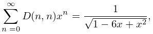
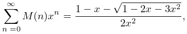
2: 26.6 Other Lattice Path Numbers

… ►For sufficiently small $|x|$ and $|y|$, ►

26.6.5 $$\sum _{m,n=0}^{\mathrm{\infty }}D(m,n)x^m{y}^n=\frac{1}{1-x-y-xy},$$

ⓘ

Symbols:

$m$: nonnegative integer, $n$: nonnegative integer, $D(m,n)$: Delannoy number, $x$: small and $y$: small

Permalink:

http://dlmf.nist.gov/26.6.E5

Encodings:

pMML, png, TeX

See also:

Annotations for §26.6(ii), §26.6 and Ch.26

►

26.6.6 $$\sum _{n=0}^{\mathrm{\infty }}D(n,n)x^n=\frac{1}{\sqrt{1-6x+x^2}},$$

ⓘ

Symbols:

$n$: nonnegative integer, $D(m,n)$: Delannoy number and $x$: small

Permalink:

http://dlmf.nist.gov/26.6.E6

Encodings:

pMML, png, TeX

See also:

Annotations for §26.6(ii), §26.6 and Ch.26

►

26.6.7 $$\sum _{n=0}^{\mathrm{\infty }}M(n)x^n=\frac{1-x-\sqrt{1-2x-3x^2}}{2x^2},$$

ⓘ

Symbols:

$n$: nonnegative integer, $M(n)$: Motzkin number and $x$: small

Referenced by:

§26.6(iii)

Permalink:

http://dlmf.nist.gov/26.6.E7

Encodings:

pMML, png, TeX

See also:

Annotations for §26.6(ii), §26.6 and Ch.26

… ►

26.6.9 $$\sum _{n=0}^{\mathrm{\infty }}r(n)x^n=\frac{1-x-\sqrt{1-6x+x^2}}{2x}.$$

ⓘ

Symbols:

$n$: nonnegative integer, $r(n)$: Schröder number and $x$: small

Permalink:

http://dlmf.nist.gov/26.6.E9

Encodings:

pMML, png, TeX

See also:

Annotations for §26.6(ii), §26.6 and Ch.26

…

3: 11.13 Methods of Computation

… ►Then from the limiting forms for small argument (§§11.2(i), 10.7(i), 10.30(i)), limiting forms for large argument (§§11.6(i), 10.7(ii), 10.30(ii)), and the connection formulas (11.2.5) and (11.2.6), it is seen that ${𝐇}_{\nu }\left(x\right)$ and ${𝐋}_{\nu }\left(x\right)$ can be computed in a stable manner by integrating forwards, that is, from the origin toward infinity. The solution ${𝐊}_{\nu }\left(x\right)$ needs to be integrated backwards for small $x$, and either forwards or backwards for large $x$ depending whether or not $\nu$ exceeds $\frac{1}{2}$. …

4: 22.16 Related Functions

… ►

Approximation for Small $x$

…

5: 36.7 Zeros

… ►Near $z=z_n$, and for small $x$ and $y$, the modulus $|{\mathrm{\Psi }}^{(\mathrm{E})}\left(𝐱\right)|$ has the symmetry of a lattice with a rhombohedral unit cell that has a mirror plane and an inverse threefold axis whose $z$ and $x$ repeat distances are given by …

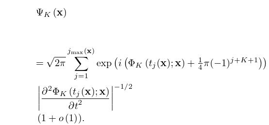
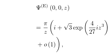
6: 36.11 Leading-Order Asymptotics

… ►

36.11.1

ⓘ

Symbols:

$t_j(𝐱)$: solutions

Permalink:

http://dlmf.nist.gov/36.11.E1

Encodings:

pMML, png, TeX

See also:

Annotations for §36.11 and Ch.36

… ►

36.11.2 $${\mathrm{\Psi }}_K\left(𝐱\right)=\sqrt{2\pi }\sum _{j=1}^{j_{\max }(𝐱)}\exp \left(\mathrm{i}\left({\mathrm{\Phi }}_K(t_j(𝐱);𝐱)+\frac{1}{4}\pi {(-1)}^{j+K+1}\right)\right){\left|\frac{{\partial }^2{\mathrm{\Phi }}_K(t_j(𝐱);𝐱)}{{\partial t}^2}\right|}^{-1/2}(1+o\left(1\right)).$$

ⓘ

Symbols:

${\mathrm{\Psi }}_K\left(𝐱\right)$: canonical integral function, $\pi$: the ratio of the circumference of a circle to its diameter, ${\mathrm{\Phi }}_K(t;𝐱)$: cuspoid catastrophe of codimension $K$ , $\exp z$: exponential function, $\mathrm{i}$: imaginary unit, $o\left(x\right)$: order less than, $\frac{\partial f}{\partial x}$: partial derivative of $f$ with respect to $x$ , $\partial x$: partial differential of $x$ , $t$: variable, $K$: codimension and $t_j(𝐱)$: solutions

Permalink:

http://dlmf.nist.gov/36.11.E2

Encodings:

pMML, png, TeX

See also:

Annotations for §36.11 and Ch.36

… ►

36.11.4

ⓘ

Symbols:

${\mathrm{\Psi }}_K\left(𝐱\right)$: canonical integral function, $\pi$: the ratio of the circumference of a circle to its diameter, $\cos z$: cosine function, $\exp z$: exponential function, $o\left(x\right)$: order less than and $x$: real parameter

Referenced by:

§36.11

Permalink:

http://dlmf.nist.gov/36.11.E4

Encodings:

pMML, png, TeX

See also:

Annotations for §36.11, §36.11 and Ch.36

►

36.11.5 $${\mathrm{\Psi }}_3\left(0,y,0\right)=\overline{{\mathrm{\Psi }}_3(0,-y,0)}=\exp \left(\frac{1}{4}\mathrm{i}\pi \right)\sqrt{\pi /y}\left(1-(\mathrm{i}/\sqrt{3})\exp \left(\frac{3}{2}\mathrm{i}{(2y/5)}^{5/3}\right)+o\left(1\right)\right),$$ $y\to +\mathrm{\infty }$.

ⓘ

Symbols:

${\mathrm{\Psi }}_K\left(𝐱\right)$: canonical integral function, $\pi$: the ratio of the circumference of a circle to its diameter, $\overline{z}$: complex conjugate, $\exp z$: exponential function, $\mathrm{i}$: imaginary unit, $o\left(x\right)$: order less than and $y$: real parameter

Permalink:

http://dlmf.nist.gov/36.11.E5

Encodings:

pMML, png, TeX

See also:

Annotations for §36.11, §36.11 and Ch.36

… ►

36.11.7 $${\mathrm{\Psi }}^{(\mathrm{E})}\left(0,0,z\right)=\frac{\pi }{z}\left(\mathrm{i}+\sqrt{3}\exp \left(\frac{4}{27}\mathrm{i}{z}^3\right)+o\left(1\right)\right),$$ $z\to \pm \mathrm{\infty }$,

ⓘ

Symbols:

$\pi$: the ratio of the circumference of a circle to its diameter, ${\mathrm{\Psi }}^{(\mathrm{E})}\left(𝐱\right)$: elliptic umbilic canonical integral function, $\exp z$: exponential function, $\mathrm{i}$: imaginary unit, $o\left(x\right)$: order less than and $z$: real parameter

Permalink:

http://dlmf.nist.gov/36.11.E7

Encodings:

pMML, png, TeX

See also:

Annotations for §36.11, §36.11 and Ch.36

…

7: 10.75 Tables

… ►

British Association for the Advancement of Science (1937) tabulates $J_0\left(x\right)$, $J_1\left(x\right)$, $x=0(.001)16(.01)25$, 10D; $Y_0\left(x\right)$, $Y_1\left(x\right)$, $x=0.01(.01)25$, 8–9S or 8D. Also included are auxiliary functions to facilitate interpolation of the tables of $Y_0\left(x\right)$, $Y_1\left(x\right)$ for small values of $x$, as well as auxiliary functions to compute all four functions for large values of $x$.

… ►

British Association for the Advancement of Science (1937) tabulates $I_0\left(x\right)$, $I_1\left(x\right)$, $x=0(.001)5$, 7–8D; $K_0\left(x\right)$, $K_1\left(x\right)$, $x=0.01(.01)5$, 7–10D; ${\mathrm{e}}^{-x}{I}_0\left(x\right)$, ${\mathrm{e}}^{-x}{I}_1\left(x\right)$, ${\mathrm{e}}^x{K}_0\left(x\right)$, ${\mathrm{e}}^x{K}_1\left(x\right)$, $x=5(.01)10(.1)20$, 8D. Also included are auxiliary functions to facilitate interpolation of the tables of $K_0\left(x\right)$, $K_1\left(x\right)$ for small values of $x$.

… ►

Young and Kirk (1964) tabulates ${\mathrm{ber}}_{n}x$, ${\mathrm{bei}}_{n}x$, ${\ker }_{n}x$, ${\mathrm{kei}}_{n}x$, $n=0,1$, $x=0(.1)10$, 15D; ${\mathrm{ber}}_{n}x$, ${\mathrm{bei}}_{n}x$, ${\ker }_{n}x$, ${\mathrm{kei}}_{n}x$, modulus and phase functions $M_n\left(x\right)$, ${\theta }_n\left(x\right)$, $N_n\left(x\right)$, ${\varphi }_n\left(x\right)$, $n=0,1,2$, $x=0(.01)2.5$, 8S, and $n=0(1)10$, $x=0(.1)10$, 7S. Also included are auxiliary functions to facilitate interpolation of the tables for $n=0(1)10$ for small values of $x$. (Concerning the phase functions see §10.68(iv).)

…

8: 10.45 Functions of Imaginary Order

… ►In consequence of (10.45.5)–(10.45.7), ${\tilde{I}}_{\nu }\left(x\right)$ and ${\tilde{K}}_{\nu }\left(x\right)$ comprise a numerically satisfactory pair of solutions of (10.45.1) when $x$ is large, and either ${\tilde{I}}_{\nu }\left(x\right)$ and $(1/\pi )\sinh \left(\pi \nu \right){\tilde{K}}_{\nu }\left(x\right)$, or ${\tilde{I}}_{\nu }\left(x\right)$ and ${\tilde{K}}_{\nu }\left(x\right)$, comprise a numerically satisfactory pair when $x$ is small, depending whether $\nu \ne 0$ or $\nu =0$. …

9: 10.24 Functions of Imaginary Order

… ►Also, in consequence of (10.24.7)–(10.24.9), when $x$ is small either ${\tilde{J}}_{\nu }\left(x\right)$ and $\tanh \left(\frac{1}{2}\pi \nu \right){\tilde{Y}}_{\nu }\left(x\right)$ or ${\tilde{J}}_{\nu }\left(x\right)$ and ${\tilde{Y}}_{\nu }\left(x\right)$ comprise a numerically satisfactory pair depending whether $\nu \ne 0$ or $\nu =0$. …

10: 4.45 Methods of Computation

… ►

4.45.9 $$x_n=\frac{x_{n-1}}{1+{(1+x_{n-1}^2)}^{1/2}},$$ $n=1,2,3,\mathrm{\dots }$,

ⓘ

Symbols:

$\arctan z$: arctangent function, $n$: integer and $x$: real variable

Referenced by:

(4.45.8), Erratum (V1.0.7) for Equations (4.45.8), (4.45.9)

Permalink:

http://dlmf.nist.gov/4.45.E9

Encodings:

pMML, png, TeX

Substitution (effective with 1.0.7):

The original recurrence given in this equation, $x_n=\frac{{(1+x_{n-1}^2)}^{1/2}-1}{x_{n-1}}$ is susceptible to cancellation error when $x_n$ is small. It has been replaced with another recurrence that is better for numerically computing $\arctan x$.

Suggested 2014-02-05 by Masataka Urago

See also:

Annotations for §4.45(i), §4.45(i), §4.45 and Ch.4

►until $x_n$ is sufficiently small. …