singularity parameter

SearchAdvancedHelp

(0.002 seconds)

1—10 of 61 matching pages

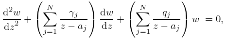
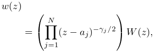
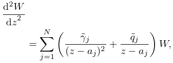
1: 31.14 General Fuchsian Equation

… ►

31.14.1 $$\frac{d^{2}w}{{dz}^2}+\left(\sum _{j=1}^N\frac{{\gamma }_j}{z-a_j}\right)\frac{dw}{dz}+\left(\sum _{j=1}^N\frac{q_j}{z-a_j}\right)w=0,$$ ${\sum }_{j=1}^N{q}_j=0$.

ⓘ

Symbols:

$\frac{df}{dx}$: derivative of $f$ with respect to $x$ , $z$: complex variable, $\gamma$: real or complex parameter, $j$: nonnegative integer, $a$: complex parameter, $q$: real or complex parameter and $N+1$: number of singularities

Referenced by:

§31.15(i)

Permalink:

http://dlmf.nist.gov/31.14.E1

Encodings:

pMML, png, TeX

See also:

Annotations for §31.14(i), §31.14 and Ch.31

… ►The three sets of parameters comprise the singularity parameters $a_j$, the exponent parameters $\alpha ,\beta ,{\gamma }_j$, and the $N-2$ free accessory parameters $q_j$. … ►

31.14.3 $$w(z)=\left(\prod _{j=1}^N{(z-a_j)}^{-{\gamma }_j/2}\right)W(z),$$

ⓘ

Symbols:

$z$: complex variable, $\gamma$: real or complex parameter, $j$: nonnegative integer, $a$: complex parameter, $N+1$: number of singularities and $W(z)$: solution

Permalink:

http://dlmf.nist.gov/31.14.E3

Encodings:

pMML, png, TeX

See also:

Annotations for §31.14(i), §31.14(i), §31.14 and Ch.31

►

31.14.4 $$\frac{d^{2}W}{{dz}^2}=\sum _{j=1}^N\left(\frac{{\tilde{\gamma }}_j}{{(z-a_j)}^2}+\frac{{\tilde{q}}_j}{z-a_j}\right)W,$$ ${\sum }_{j=1}^N{\tilde{q}}_j=0$,

ⓘ

Defines:

$W(z)$: solution (locally)

Symbols:

$\frac{df}{dx}$: derivative of $f$ with respect to $x$ , $z$: complex variable, $\gamma$: real or complex parameter, $j$: nonnegative integer, $a$: complex parameter, $q$: real or complex parameter and $N+1$: number of singularities

Permalink:

http://dlmf.nist.gov/31.14.E4

Encodings:

pMML, png, TeX

See also:

Annotations for §31.14(i), §31.14(i), §31.14 and Ch.31

…

2: 31.2 Differential Equations

… ►

31.2.1 $$\frac{d^{2}w}{{dz}^2}+\left(\frac{\gamma }{z}+\frac{\delta }{z-1}+\frac{ϵ}{z-a}\right)\frac{dw}{dz}+\frac{\alpha \beta z-q}{z(z-1)(z-a)}w=0,$$ $\alpha +\beta +1=\gamma +\delta +ϵ$.

ⓘ

Symbols:

$\frac{df}{dx}$: derivative of $f$ with respect to $x$ , $z$: complex variable, $\gamma$: real or complex parameter, $\delta$: real or complex parameter, $ϵ$: real or complex parameter, $a$: complex parameter, $q$: real or complex parameter, $\alpha$: real or complex parameter and $\beta$: real or complex parameter

Referenced by:

§29.2(ii), §31.11(iii), §31.12, §31.13, §31.14(i), §31.17(i), §31.18, §31.2(v), §31.2(v), §31.2(v), §31.2(i), §31.3(i), §31.3(i), §31.3(ii), §31.3(ii), §31.3(ii), §31.3(iii), §31.3(iii), §31.4, §31.5, §31.6, §31.7(ii), §31.8, §31.8, §31.8

Permalink:

http://dlmf.nist.gov/31.2.E1

Encodings:

pMML, png, TeX

See also:

Annotations for §31.2(i), §31.2 and Ch.31

… ►All other homogeneous linear differential equations of the second order having four regular singularities in the extended complex plane, $ℂ\cup \{\mathrm{\infty }\}$, can be transformed into (31.2.1). ►The parameters play different roles: $a$ is the singularity parameter; $\alpha ,\beta ,\gamma ,\delta ,ϵ$ are exponent parameters; $q$ is the accessory parameter. …

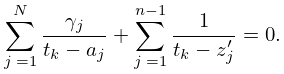
3: 31.15 Stieltjes Polynomials

… ►

31.15.3 $$\sum _{j=1}^N\frac{{\gamma }_j}{t_k-a_j}+\sum _{j=1}^{n-1}\frac{1}{t_k-z_j^{\prime }}=0.$$

ⓘ

Symbols:

$z$: complex variable, $\gamma$: real or complex parameter, $j$: nonnegative integer, $n$: nonnegative integer, $a$: complex parameter, $N+1$: number of singularities and $t_k$: zero of $V(z)$

Permalink:

http://dlmf.nist.gov/31.15.E3

Encodings:

pMML, png, TeX

See also:

Annotations for §31.15(ii), §31.15 and Ch.31

… ►

31.15.6 $j=1,2,\mathrm{\dots },N-1$,

ⓘ

Symbols:

$j$: nonnegative integer, $a$: complex parameter and $N+1$: number of singularities

Referenced by:

§31.15(iii)

Permalink:

http://dlmf.nist.gov/31.15.E6

Encodings:

pMML, png, TeX

See also:

Annotations for §31.15(ii), §31.15 and Ch.31

… ►

31.15.7 $$q_j={\gamma }_j\sum _{k=1}^n\frac{1}{z_k-a_j},$$ $j=1,2,\mathrm{\dots },N$.

ⓘ

Symbols:

$z$: complex variable, $\gamma$: real or complex parameter, $j$: nonnegative integer, $n$: nonnegative integer, $a$: complex parameter, $q$: real or complex parameter and $N+1$: number of singularities

Permalink:

http://dlmf.nist.gov/31.15.E7

Encodings:

pMML, png, TeX

See also:

Annotations for §31.15(ii), §31.15 and Ch.31

… ►If the exponent and singularity parameters satisfy (31.15.5)–(31.15.6), then for every multi-index $𝐦=(m_1,m_2,\mathrm{\dots },m_{N-1})$, where each $m_j$ is a nonnegative integer, there is a unique Stieltjes polynomial with $m_j$ zeros in the open interval $(a_j,a_{j+1})$ for each $j=1,2,\mathrm{\dots },N-1$. … ►

31.15.8 $$S_{𝐦}(z_1)S_{𝐦}(z_2)\mathrm{\cdots }{S}_{𝐦}(z_{N-1}),$$ $z_j\in (a_j,a_{j+1})$,

ⓘ

Symbols:

$\in$: element of, $(a,b)$: open interval, $z$: complex variable, $j$: nonnegative integer, $a$: complex parameter, $N+1$: number of singularities and $S_{𝐦}(z)$: Stieltjes polynomial

Referenced by:

§31.15(iii)

Permalink:

http://dlmf.nist.gov/31.15.E8

Encodings:

pMML, png, TeX

See also:

Annotations for §31.15(iii), §31.15 and Ch.31

…

4: 31.13 Asymptotic Approximations

§31.13 Asymptotic Approximations

►For asymptotic approximations for the accessory parameter eigenvalues $q_m$, see Fedoryuk (1991) and Slavyanov (1996). ►For asymptotic approximations of the solutions of Heun’s equation (31.2.1) when two singularities are close together, see Lay and Slavyanov (1999). ►For asymptotic approximations of the solutions of confluent forms of Heun’s equation in the neighborhood of irregular singularities, see Komarov et al. (1976), Ronveaux (1995, Parts B,C,D,E), Bogush and Otchik (1997), Slavyanov and Veshev (1997), and Lay et al. (1998).

5: 2.4 Contour Integrals

… ►For a coalescing saddle point and endpoint see Olver (1997b, Chapter 9) and Wong (1989, Chapter 7); if the endpoint is an algebraic singularity then the uniform approximants are parabolic cylinder functions with fixed parameter, and if the endpoint is not a singularity then the uniform approximants are complementary error functions. …

6: 31.1 Special Notation

… ►Sometimes the parameters are suppressed.

7: 30.2 Differential Equations

… ►This equation has regular singularities at $z=\pm 1$ with exponents $\pm \frac{1}{2}\mu$ and an irregular singularity of rank 1 at $z=\mathrm{\infty }$ (if $\gamma \ne 0$). The equation contains three real parameters $\lambda$, ${\gamma }^2$, and $\mu$. … … ►

30.2.2 $$\frac{d^{2}g}{{dt}^2}+\left(\lambda +\frac{1}{4}+{\gamma }^2{\sin }^{2}t-\frac{{\mu }^2-\frac{1}{4}}{{\sin }^{2}t}\right)g=0,$$

ⓘ

Symbols:

$\frac{df}{dx}$: derivative of $f$ with respect to $x$ , $\sin z$: sine function, $\lambda$: real parameter, ${\gamma }^2$: real parameter and $\mu$: real parameter

Referenced by:

§30.2(iii)

Permalink:

http://dlmf.nist.gov/30.2.E2

Encodings:

pMML, png, TeX

See also:

Annotations for §30.2(ii), §30.2 and Ch.30

… ►With $\zeta =\gamma z$ Equation (30.2.1) changes to …

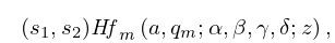
8: 31.11 Expansions in Series of Hypergeometric Functions

… ►

31.11.3 $$\lambda +\mu =\gamma +\delta -1=\alpha +\beta -ϵ.$$

ⓘ

Defines:

$\lambda$ (locally) and $\mu$ (locally)

Symbols:

$\gamma$: real or complex parameter, $\delta$: real or complex parameter, $ϵ$: real or complex parameter, $\alpha$: real or complex parameter and $\beta$: real or complex parameter

Permalink:

http://dlmf.nist.gov/31.11.E3

Encodings:

pMML, png, TeX

See also:

Annotations for §31.11(ii), §31.11 and Ch.31

… ►and (31.11.1) converges to (31.3.10) outside the ellipse $ℰ$ in the $z$-plane with foci at 0, 1, and passing through the third finite singularity at $z=a$. ►Every Heun function (§31.4) can be represented by a series of Type I convergent in the whole plane cut along a line joining the two singularities of the Heun function. … ►The expansion (31.11.1) with (31.11.12) is convergent in the plane cut along the line joining the two singularities $z=0$ and $z=1$. In this case the accessory parameter $q$ is a root of the continued-fraction equation …

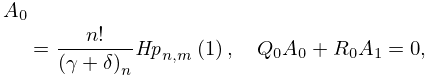
9: 31.4 Solutions Analytic at Two Singularities: Heun Functions

§31.4 Solutions Analytic at Two Singularities: Heun Functions

►For an infinite set of discrete values $q_m$, $m=0,1,2,\mathrm{\dots }$, of the accessory parameter $q$, the function $H\mathrm{\ell }(a,q;\alpha ,\beta ,\gamma ,\delta ;z)$ is analytic at $z=1$, and hence also throughout the disk . … ►

31.4.1 $$(0,1){\mathrm{𝐻𝑓}}_m(a,q_m;\alpha ,\beta ,\gamma ,\delta ;z),$$ $m=0,1,2,\mathrm{\dots }$.

ⓘ

Symbols:

$(s_1,s_2){\mathrm{𝐻𝑓}}_m(a,q_m;\alpha ,\beta ,\gamma ,\delta ;z)$: Heun functions, $z$: complex variable, $\gamma$: real or complex parameter, $\delta$: real or complex parameter, $m$: nonnegative integer, $a$: complex parameter, $q$: real or complex parameter, $\alpha$: real or complex parameter and $\beta$: real or complex parameter

Referenced by:

§31.6

Permalink:

http://dlmf.nist.gov/31.4.E1

Encodings:

pMML, png, TeX

See also:

Annotations for §31.4 and Ch.31

►The eigenvalues $q_m$ satisfy the continued-fraction equation … ►

31.4.3 $$(s_1,s_2){\mathrm{𝐻𝑓}}_m(a,q_m;\alpha ,\beta ,\gamma ,\delta ;z),$$ $m=0,1,2,\mathrm{\dots }$,

ⓘ

Symbols:

$(s_1,s_2){\mathrm{𝐻𝑓}}_m(a,q_m;\alpha ,\beta ,\gamma ,\delta ;z)$: Heun functions, $z$: complex variable, $\gamma$: real or complex parameter, $\delta$: real or complex parameter, $m$: nonnegative integer, $a$: complex parameter, $q$: real or complex parameter, $\alpha$: real or complex parameter and $\beta$: real or complex parameter

Referenced by:

§31.4, §31.6

Permalink:

http://dlmf.nist.gov/31.4.E3

Encodings:

pMML, png, TeX

See also:

Annotations for §31.4 and Ch.31

…

10: 31.16 Mathematical Applications

… ► thesis “Inversion problem for a second-order linear differential equation with four singular points”. It describes the monodromy group of Heun’s equation for specific values of the accessory parameter. … ►

31.16.3 $$A_0=\frac{n!}{{\left(\gamma +\delta \right)}_n}{\mathrm{𝐻𝑝}}_{n,m}\left(1\right),Q_0{A}_0+R_0{A}_1=0,$$

ⓘ

Symbols:

${\mathrm{𝐻𝑝}}_{n,m}(a,q_{n,m};-n,\beta ,\gamma ,\delta ;z)$: Heun polynomials, ${\left(a\right)}_n$: Pochhammer’s symbol (or shifted factorial), $!$: factorial (as in $n!$), $\gamma$: real or complex parameter, $\delta$: real or complex parameter, $m$: nonnegative integer, $n$: nonnegative integer, $a$: complex parameter, $q$: real or complex parameter, $\beta$: real or complex parameter, $A_j$: coefficients, $Q_j$ and $R_j$

Referenced by:

§31.16(ii), Erratum (V1.0.21) for Equations (31.16.2) and (31.16.3), Erratum (V1.0.21) for Equations (31.16.2) and (31.16.3)

Permalink:

http://dlmf.nist.gov/31.16.E3

Encodings:

pMML, png, TeX

Correction (effective with 1.0.21):

The initial data $A_0$, previously missing, has now been included.

See also:

Annotations for §31.16(ii), §31.16 and Ch.31

… ►

31.16.5 $$P_j=\frac{(ϵ-j+n)j(\beta +j-1)(\gamma +\delta +j-2)}{(\gamma +\delta +2j-3)(\gamma +\delta +2j-2)},$$

ⓘ

Defines:

$P_j$ (locally)

Symbols:

$\gamma$: real or complex parameter, $\delta$: real or complex parameter, $ϵ$: real or complex parameter, $j$: nonnegative integer, $n$: nonnegative integer and $\beta$: real or complex parameter

Permalink:

http://dlmf.nist.gov/31.16.E5

Encodings:

pMML, png, TeX

See also:

Annotations for §31.16(ii), §31.16 and Ch.31

►

31.16.6 $$Q_j=-aj(j+\gamma +\delta -1)-q+\frac{(j-n)(j+\beta )(j+\gamma )(j+\gamma +\delta -1)}{(2j+\gamma +\delta )(2j+\gamma +\delta -1)}+\frac{(j+n+\gamma +\delta -1)j(j+\delta -1)(j-\beta +\gamma +\delta -1)}{(2j+\gamma +\delta -1)(2j+\gamma +\delta -2)},$$

ⓘ

Defines:

$Q_j$ (locally)

Symbols:

$\gamma$: real or complex parameter, $\delta$: real or complex parameter, $j$: nonnegative integer, $n$: nonnegative integer, $a$: complex parameter, $q$: real or complex parameter and $\beta$: real or complex parameter

Permalink:

http://dlmf.nist.gov/31.16.E6

Encodings:

pMML, png, TeX

See also:

Annotations for §31.16(ii), §31.16 and Ch.31

…