several variables

SearchAdvancedHelp

(0.001 seconds)

11—20 of 34 matching pages

11: 1.14 Integral Transforms

… ►The same notation $ℱ$ is used for Fourier transforms of functions of several variables and for Fourier transforms of distributions; see §1.16(vii). …

12: Bibliography B

… ►

Several Complex Variables. Princeton Mathematical Series, Vol. 10, Princeton University Press, Princeton, N.J..

ⓘ

External Links:

MathReview (P. Thullen), ZentralBlatt

Referenced by:

§35.2.

Encodings:

BibTeX

…

13: 2.3 Integrals of a Real Variable

§2.3 Integrals of a Real Variable

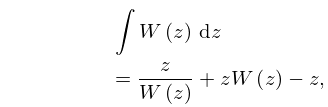
… ► $k$ ($\le \mathrm{\infty }$) and $\lambda$ are positive constants, $\alpha$ is a variable parameter in an interval ${\alpha }_1\le \alpha \le {\alpha }_2$ with ${\alpha }_1\le 0$ and , and $x$ is a large positive parameter. …In consequence, the approximation is nonuniform with respect to $\alpha$ and deteriorates severely as $\alpha \to 0$. ►A uniform approximation can be constructed by quadratic change of integration variable: ►

2.3.25 $$p(\alpha ,t)=\frac{1}{2}{w}^2-aw+b,$$

ⓘ

Symbols:

$p(\alpha ,t)$: function, $w$: change of variable, $a(\alpha )$ and $b(\alpha )$

Permalink:

http://dlmf.nist.gov/2.3.E25

Encodings:

pMML, png, TeX

See also:

Annotations for §2.3(v), §2.3 and Ch.2

…

14: 4.13 Lambert $W$-Function

… ►

4.13.1 $$W{\mathrm{e}}^W=z.$$

ⓘ

Defines:

$W\left(z\right)$: Lambert $W$-function

Symbols:

$\mathrm{e}$: base of natural logarithm and $z$: complex variable

Referenced by:

§4.13

Permalink:

http://dlmf.nist.gov/4.13.E1

Encodings:

pMML, png, TeX

See also:

Annotations for §4.13 and Ch.4

… ►

4.13.1_2 $$\omega \left(z\right)+\ln \left(\omega \left(z\right)\right)=z,$$

ⓘ

Symbols:

$\omega \left(z\right)$: Wright $\omega$-function, $\ln z$: principal branch of logarithm function and $z$: complex variable

Referenced by:

(4.13.3), §4.13, Erratum (V1.1.7) for Expansion

Permalink:

http://dlmf.nist.gov/4.13.E1_2

Encodings:

pMML, png, TeX

Rearrangement (effective with 1.1.7):

This equation, which was originally (4.13.3), was moved here, and the symbol for $\omega$ was originally $U$.

See also:

Annotations for §4.13 and Ch.4

►and has several advantages over the Lambert $W$-function (see Lawrence et al. (2012)), and the tree $T$-function $T\left(z\right)=-W\left(-z\right)$, which is a solution of ►

4.13.1_3 $$T{\mathrm{e}}^{-T}=z.$$

ⓘ

Symbols:

$T\left(z\right)$: Tree $T$-function, $\mathrm{e}$: base of natural logarithm and $z$: complex variable

Referenced by:

§4.13, Erratum (V1.1.7) for Expansion

Permalink:

http://dlmf.nist.gov/4.13.E1_3

Encodings:

pMML, png, TeX

Addition (effective with 1.1.7):

This equation was added.

See also:

Annotations for §4.13 and Ch.4

… ►

4.13.12 $$\int W\left(z\right)dz=\frac{z}{W\left(z\right)}+zW\left(z\right)-z,$$

ⓘ

Symbols:

$W\left(z\right)$: Lambert $W$-function, $dx$: differential of $x$ , $\int$: integral and $z$: complex variable

Permalink:

http://dlmf.nist.gov/4.13.E12

Encodings:

pMML, png, TeX

Addition (effective with 1.1.7):

This equation was added.

See also:

Annotations for §4.13 and Ch.4

…

15: Annie A. M. Cuyt

… ►Subsequently she was a Research fellow with the Alexander von Humboldt Foundation (Germany), she obtained the Habilitation (1986) and became author or co-author of several books, including Handbook of Continued Fractions for Special Functions. …A lot of her research has been devoted to rational approximations, in one as well as in many variables, and sparse interpolation. …

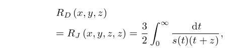
16: 19.16 Definitions

… ►A fourth integral that is symmetric in only two variables is defined by ►

19.16.5 $$R_D(x,y,z)=R_J(x,y,z,z)=\frac{3}{2}{\int }_0^{\mathrm{\infty }}\frac{dt}{s(t)(t+z)},$$

ⓘ

Defines:

$R_D(x,y,z)$: elliptic integral symmetric in only two variables

Symbols:

$R_J(x,y,z,p)$: symmetric elliptic integral of third kind, $dx$: differential of $x$ , $\int$: integral and $s(t)$: scaling factor

Referenced by:

§19.18(i), §19.19, §19.20(iii), §19.20(iv), §19.24(ii), §19.6(iv)

Permalink:

http://dlmf.nist.gov/19.16.E5

Encodings:

pMML, png, TeX

See also:

Annotations for §19.16(i), §19.16 and Ch.19

… ►Thus $R_{-a}(𝐛;𝐳)$ is symmetric in the variables $z_j$ and $z_{\mathrm{\ell }}$ if the parameters $b_j$ and $b_{\mathrm{\ell }}$ are equal. The $R$-function is often used to make a unified statement of a property of several elliptic integrals. … ►When one variable is 0 without destroying convergence, any one of (19.16.14)–(19.16.17) is said to be complete and can be written as an $R$-function with one less variable: …

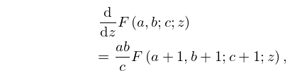
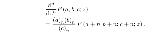
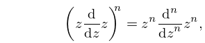
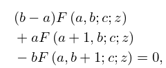
17: 15.5 Derivatives and Contiguous Functions

… ►

15.5.1 $$\frac{d}{dz}F(a,b;c;z)=\frac{ab}{c}F(a+1,b+1;c+1;z),$$

ⓘ

Symbols:

$F(a,b;c;z)$ or $F(\genfrac{}{}{0pt}{}{a,b}{c};z)$: $={}_2{}^{}F_1^{}(a,b;c;z)$ Gauss’ hypergeometric function, $\frac{df}{dx}$: derivative of $f$ with respect to $x$ , $z$: complex variable, $a$: real or complex parameter, $b$: real or complex parameter and $c$: real or complex parameter

Permalink:

http://dlmf.nist.gov/15.5.E1

Encodings:

pMML, png, TeX

See also:

Annotations for §15.5(i), §15.5 and Ch.15

►

15.5.2 $$\frac{d^n}{{dz}^n}F(a,b;c;z)=\frac{{\left(a\right)}_n{\left(b\right)}_n}{{\left(c\right)}_n}F(a+n,b+n;c+n;z).$$

ⓘ

Symbols:

$F(a,b;c;z)$ or $F(\genfrac{}{}{0pt}{}{a,b}{c};z)$: $={}_2{}^{}F_1^{}(a,b;c;z)$ Gauss’ hypergeometric function, ${\left(a\right)}_n$: Pochhammer’s symbol (or shifted factorial), $\frac{df}{dx}$: derivative of $f$ with respect to $x$ , $n$: integer, $z$: complex variable, $a$: real or complex parameter, $b$: real or complex parameter and $c$: real or complex parameter

Permalink:

http://dlmf.nist.gov/15.5.E2

Encodings:

pMML, png, TeX

See also:

Annotations for §15.5(i), §15.5 and Ch.15

… ►Other versions of several of the identities in this subsection can be constructed with the aid of the operator identity ►

15.5.10 $${\left(z\frac{d}{dz}z\right)}^n=z^n\frac{d^n}{{dz}^n}{z}^n,$$ $n=1,2,3,\mathrm{\dots }$.

ⓘ

Symbols:

$\frac{df}{dx}$: derivative of $f$ with respect to $x$ , $n$: integer and $z$: complex variable

Referenced by:

§15.5(i)

Permalink:

http://dlmf.nist.gov/15.5.E10

Encodings:

pMML, png, TeX

See also:

Annotations for §15.5(i), §15.5 and Ch.15

… ►

15.5.12 $$(b-a)F(a,b;c;z)+aF(a+1,b;c;z)-bF(a,b+1;c;z)=0,$$

ⓘ

Symbols:

$F(a,b;c;z)$ or $F(\genfrac{}{}{0pt}{}{a,b}{c};z)$: $={}_2{}^{}F_1^{}(a,b;c;z)$ Gauss’ hypergeometric function, $z$: complex variable, $a$: real or complex parameter, $b$: real or complex parameter and $c$: real or complex parameter

Permalink:

http://dlmf.nist.gov/15.5.E12

Encodings:

pMML, png, TeX

See also:

Annotations for §15.5(ii), §15.5 and Ch.15

…

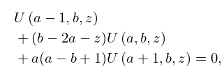
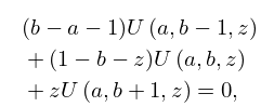
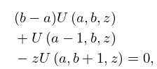
18: 13.3 Recurrence Relations and Derivatives

… ►

13.3.7 $$U(a-1,b,z)+(b-2a-z)U(a,b,z)+a(a-b+1)U(a+1,b,z)=0,$$

ⓘ

Symbols:

$U(a,b,z)$: Kummer confluent hypergeometric function and $z$: complex variable

A&S Ref:

13.4.15

Permalink:

http://dlmf.nist.gov/13.3.E7

Encodings:

pMML, png, TeX

See also:

Annotations for §13.3(i), §13.3 and Ch.13

►

13.3.8 $$(b-a-1)U(a,b-1,z)+(1-b-z)U(a,b,z)+zU(a,b+1,z)=0,$$

ⓘ

Symbols:

$U(a,b,z)$: Kummer confluent hypergeometric function and $z$: complex variable

A&S Ref:

13.4.16

Permalink:

http://dlmf.nist.gov/13.3.E8

Encodings:

pMML, png, TeX

See also:

Annotations for §13.3(i), §13.3 and Ch.13

►

13.3.9 $$U(a,b,z)-aU(a+1,b,z)-U(a,b-1,z)=0,$$

ⓘ

Symbols:

$U(a,b,z)$: Kummer confluent hypergeometric function and $z$: complex variable

A&S Ref:

13.4.17

Permalink:

http://dlmf.nist.gov/13.3.E9

Encodings:

pMML, png, TeX

See also:

Annotations for §13.3(i), §13.3 and Ch.13

►

13.3.10 $$(b-a)U(a,b,z)+U(a-1,b,z)-zU(a,b+1,z)=0,$$

ⓘ

Symbols:

$U(a,b,z)$: Kummer confluent hypergeometric function and $z$: complex variable

A&S Ref:

13.4.18

Permalink:

http://dlmf.nist.gov/13.3.E10

Encodings:

pMML, png, TeX

See also:

Annotations for §13.3(i), §13.3 and Ch.13

… ►Other versions of several of the identities in this subsection can be constructed with the aid of the operator identity …

19: 5.4 Special Values and Extrema

… ►

5.4.3 $$|\mathrm{\Gamma }\left(\mathrm{i}y\right)|={\left(\frac{\pi }{y\sinh \left(\pi y\right)}\right)}^{1/2},$$

ⓘ

Symbols:

$\mathrm{\Gamma }\left(z\right)$: gamma function, $\pi$: the ratio of the circumference of a circle to its diameter, $\sinh z$: hyperbolic sine function, $\mathrm{i}$: imaginary unit and $y$: real variable

A&S Ref:

6.1.29

Referenced by:

§10.24, §5.4(i)

Permalink:

http://dlmf.nist.gov/5.4.E3

Encodings:

pMML, png, TeX

See also:

Annotations for §5.4(i), §5.4 and Ch.5

… ►

5.4.16 $$\mathrm{\Im }\psi \left(\mathrm{i}y\right)=\frac{1}{2y}+\frac{\pi }{2}\coth \left(\pi y\right),$$

ⓘ

Symbols:

$\pi$: the ratio of the circumference of a circle to its diameter, $\psi \left(z\right)$: psi (or digamma) function, $\coth z$: hyperbolic cotangent function, $\mathrm{\Im }$: imaginary part, $\mathrm{i}$: imaginary unit and $y$: real variable

A&S Ref:

6.3.11

Permalink:

http://dlmf.nist.gov/5.4.E16

Encodings:

pMML, png, TeX

See also:

Annotations for §5.4(ii), §5.4 and Ch.5

►

5.4.17 $$\mathrm{\Im }\psi \left(\frac{1}{2}+\mathrm{i}y\right)=\frac{\pi }{2}\tanh \left(\pi y\right),$$

ⓘ

Symbols:

$\pi$: the ratio of the circumference of a circle to its diameter, $\psi \left(z\right)$: psi (or digamma) function, $\tanh z$: hyperbolic tangent function, $\mathrm{\Im }$: imaginary part, $\mathrm{i}$: imaginary unit and $y$: real variable

A&S Ref:

6.3.12

Permalink:

http://dlmf.nist.gov/5.4.E17

Encodings:

pMML, png, TeX

See also:

Annotations for §5.4(ii), §5.4 and Ch.5

►

5.4.18 $$\mathrm{\Im }\psi \left(1+\mathrm{i}y\right)=-\frac{1}{2y}+\frac{\pi }{2}\coth \left(\pi y\right).$$

ⓘ

Symbols:

$\pi$: the ratio of the circumference of a circle to its diameter, $\psi \left(z\right)$: psi (or digamma) function, $\coth z$: hyperbolic cotangent function, $\mathrm{\Im }$: imaginary part, $\mathrm{i}$: imaginary unit and $y$: real variable

A&S Ref:

6.3.13

Referenced by:

§5.4(ii)

Permalink:

http://dlmf.nist.gov/5.4.E18

Encodings:

pMML, png, TeX

See also:

Annotations for §5.4(ii), §5.4 and Ch.5

… ►

5.4.20 $$x_n=-n+\frac{1}{\pi }\arctan \left(\frac{\pi }{\ln n}\right)+O\left(\frac{1}{n{(\ln n)}^2}\right).$$

ⓘ

Symbols:

$O\left(x\right)$: order not exceeding, $\pi$: the ratio of the circumference of a circle to its diameter, $\arctan z$: arctangent function, $\ln z$: principal branch of logarithm function, $n$: nonnegative integer and $x$: real variable

A&S Ref:

6.3.20 (The error estimate has been improved.)

Referenced by:

§5.4(iii)

Permalink:

http://dlmf.nist.gov/5.4.E20

Encodings:

pMML, png, TeX

See also:

Annotations for §5.4(iii), §5.4 and Ch.5

…

20: Errata

… ►

The following additions were made in Chapter 18:

• In Subsection 18.2(i), Equation (18.2.1_5); the paragraph title “Orthogonality on Finite Point Sets” has been changed to “Orthogonality on Countable Sets”, and there are minor changes in the presentation of the final paragraph, including a new equation (18.2.4_5). The presentation of Subsection 18.2(iii) has changed, Equation (18.2.5_5) was added and an extra paragraph on standardizations has been included. The presentation of Subsection 18.2(iv) has changed and it has been expanded with two extra paragraphs and several new equations, (18.2.9_5), (18.2.11_1)–(18.2.11_9). Subsections 18.2(v) (with (18.2.12_5), (18.2.14)–(18.2.17)) and 18.2(vi) (with (18.2.17)–(18.2.20)) have been expanded. New subsections, 18.2(vii)–18.2(xii), with Equations (18.2.21)–(18.2.46),

• A new introduction, minor changes in the presentation, and three new paragraphs.

• Extra details for Chebyshev polynomials, and Equations (18.5.4_5), (18.5.11_1)–(18.5.11_4), (18.5.17_5).

• Line numbers and two extra rows were added to Table 18.8.1.

• Subsection 18.9(i) has been expanded, and 18.9(iii) has some additional explanation. Equations (18.9.2_1), (18.9.2_2), (18.9.18_5) and Table 18.9.2 were added.

• Three extra generating functions, (18.12.2_5), (18.12.3_5), (18.12.17).

• Equation (18.14.3_5). New subsection, 18.14(iv), with Equations (18.14.25)–(18.14.27).

• Equation (18.15.4_5).

• The title of Subsection 18.16(iii) was changed from “Ultraspherical and Legendre” to “Ultraspherical, Legendre and Chebyshev”. New subsection, 18.16(vii) Discriminants, with Equations (18.16.19)–(18.16.21).

• Extra explanatory text at many places and seven extra integrals (18.17.16_5), (18.17.21_1)–(18.17.21_3), (18.17.28_5), (18.17.34_5), (18.17.41_5).

• Extra explanatory text at several places and the title of Subsection 18.18(iv) was changed from “Connection Formulas” to “Connection and Inversion Formulas”.

• A new introduction.

• Equation (18.21.13).

• Extra explanatory text in Subsection 18.25(i) and the title of Subsection 18.25(ii) was changed from “Weights and Normalizations: Continuous Cases” to “Weights and Standardizations: Continuous Cases”.

• In Subsection 18.26(i) an extra paragraph on dualities has been included, with Equations (18.26.4_1), (18.26.4_2).

• Extra text at the start of this section and twenty seven extra formulas, (18.27.4_1), (18.27.4_2), (18.27.6_5), (18.27.9_5), (18.27.12_5), (18.27.14_1)–(18.27.14_6), (18.27.17_1)–(18.27.17_3), (18.27.20_5), (18.27.25), (18.27.26), (18.28.1_5).

• A big expansion. Six extra formulas in Subsection 18.28(ii) ((18.28.6_1)–(18.28.6_5)) and three extra formulas in Subsection 18.28(viii) ((18.28.21)–(18.28.23)). New subsections, 18.28(ix)–18.28(xi), with Equations (18.28.23)–(18.28.34).

• Originally this section did not have subsections. The original seven formulas have now more explanatory text and are split over two subsections. New subsections 18.30(iii)–18.30(viii), with Equations (18.30.8)–(18.30.31).

• This short section has been expanded, with Equation (18.32.2).

• Additional references and a new large subsection, 18.33(vi), including Equations (18.33.17)–(18.33.32).

• This section has been expanded, including an extra orthogonality relations (18.34.5_5), (18.34.7_1)–(18.34.7_3).

• This section on Pollaczek polynomials has been significantly updated with much more explanations and as well to include the Pollaczek polynomials of type 3 which are the most general with three free parameters. The Pollaczek polynomials which were previously treated, namely those of type 1 and type 2 are special cases of the type 3 Pollaczek polynomials. In the first paragraph of this section an extensive description of the relations between the three types of Pollaczek polynomials is given which was lacking previously. Equations (18.35.0_5), (18.35.2_1)–(18.35.2_5), (18.35.4_5), (18.35.6_1)–(18.35.6_6), (18.35.10).

• This section on miscellaneous polynomials has been expanded with new subsections, 18.36(v) on non-classical Laguerre polynomials and 18.36(vi) with examples of exceptional orthogonal polynomials, with Equations (18.36.1)–(18.36.10). In the titles of Subsections 18.36(ii) and 18.36(iii) we replaced “OP’s” by “Orthogonal Polynomials”.

• The paragraphs of Subsection 18.38(i) have been re-ordered and one paragraph was added. The title of Subsection 18.38(ii) was changed from “Classical OP’s: Other Applications” to “Classical OP’s: Mathematical Developments and Applications”. Subsection 18.38(iii) has been expanded with seven new paragraphs, and Equations (18.38.4)–(18.38.11).

• This section was completely rewritten. The previous 18.39(i) Quantum Mechanics has been replaced by Subsections 18.39(i) Quantum Mechanics and 18.39(ii) A 3D Separable Quantum System, the Hydrogen Atom, containing the same essential information; the original content of the subsection is reproduced below for reference. Subsection 18.39(ii) was moved to 18.39(v) Other Applications. New subsections, 18.39(iii) Non Classical Weight Functions of Utility in DVR Method in the Physical Sciences, 18.39(iv) Coulomb–Pollaczek Polynomials and J-Matrix Methods; Equations (18.39.7)–(18.39.48); and Figures 18.39.1, 18.39.2.

  The original text of 18.39(i) Quantum Mechanics was:

  “Classical OP’s appear when the time-dependent Schrödinger equation is solved by separation of variables. Consider, for example, the one-dimensional form of this equation for a particle of mass $m$ with potential energy $V(x)$:

  errata.1 $$\left(\frac{-{\mathrm{\hslash }}^2}{2m}\frac{{\partial }^2}{{\partial x}^2}+V(x)\right)\psi (x,t)=i\mathrm{\hslash }\frac{\partial }{\partial t}\psi (x,t),$$

  where $\mathrm{\hslash }$ is the reduced Planck’s constant. On substituting $\psi (x,t)=\eta (x)\zeta (t)$, we obtain two ordinary differential equations, each of which involve the same constant $E$. The equation for $\eta (x)$ is

  errata.2 $$\frac{d^2\eta }{{dx}^2}+\frac{2m}{{\mathrm{\hslash }}^2}\left(E-V(x)\right)\eta =0.$$

  For a harmonic oscillator, the potential energy is given by

  errata.3 $$V(x)=\frac{1}{2}m{\omega }^2{x}^2,$$

  where $\omega$ is the angular frequency. For (18.39.2) to have a nontrivial bounded solution in the interval , the constant $E$ (the total energy of the particle) must satisfy

  errata.4 $$E=E_n=\left(n+\frac{1}{2}\right)\mathrm{\hslash }\omega ,$$ $n=0,1,2,\mathrm{\dots }$.

  The corresponding eigenfunctions are

  errata.5 $${\eta }_n(x)={\pi }^{-\frac{1}{4}}{2}^{-\frac{1}{2}n}{(n!b)}^{-\frac{1}{2}}{H}_n\left(x/b\right){\mathrm{e}}^{-x^2/2b^2},$$

  where $b={(\mathrm{\hslash }/m\omega )}^{1/2}$, and $H_n$ is the Hermite polynomial. For further details, see Seaborn (1991, p. 224) or Nikiforov and Uvarov (1988, pp. 71-72).

  A second example is provided by the three-dimensional time-independent Schrödinger equation

  errata.6 $${\nabla }^2\psi +\frac{2m}{{\mathrm{\hslash }}^2}\left(E-V(𝐱)\right)\psi =0,$$

  when this is solved by separation of variables in spherical coordinates (§1.5(ii)). The eigenfunctions of one of the separated ordinary differential equations are Legendre polynomials. See Seaborn (1991, pp. 69-75).

  For a third example, one in which the eigenfunctions are Laguerre polynomials, see Seaborn (1991, pp. 87-93) and Nikiforov and Uvarov (1988, pp. 76-80 and 320-323).”

• The old section is now Subsection 18.40(i) and a large new subsection, 18.40(ii), on the classical moment problem has been added, with formulae (18.40.1)–(18.40.10) and Figures 18.40.1, 18.40.2.

… ►

Several changes have been made to

1. make consistent use of the Fourier transform notations $ℱ\left(f\right)$, $ℱ\left(\varphi \right)$ and $ℱ\left(u\right)$ where $f$ is a function of one real variable, $\varphi$ is a test function of $n$ variables associated with tempered distributions, and $u$ is a tempered distribution (see (1.14.1), (1.16.29) and (1.16.35));

2. introduce the partial differential operator $𝐃$ in (1.16.30);

3. clarify the definition (1.16.32) of the partial differential operator $P(𝐃)$; and

4. clarify the use of $P(𝐃)$ and $P(𝐱)$ in (1.16.33), (1.16.34), (1.16.36) and (1.16.37).

…