scaled

SearchAdvancedHelp

(0.001 seconds)

21—30 of 61 matching pages

21: Viewing DLMF Interactive 3D Graphics

… ►Users can render a 3D scene and interactively rotate, scale, and otherwise explore a function surface. …

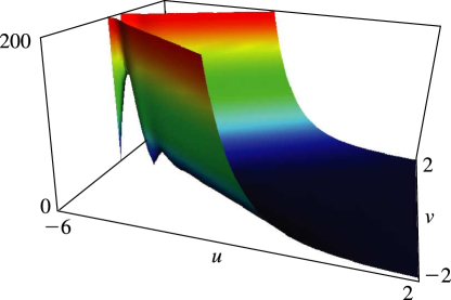
22: 15.3 Graphics

… ►

►

►

Figure 15.3.7: $|𝐅(-3,\frac{3}{5};u+\mathrm{i}v;\frac{1}{2})|,-6\le u\le 2,-2\le v\le 2$. Magnify 3D Help

23: About Color Map

… ►Mathematically, we scale the height to $h$ lying in the interval $[0,4]$ and the components are computed as follows … ►Specifically, by scaling the phase angle in $[0,2\pi )$ to $q$ in the interval $[0,4)$, the hue (in degrees) is computed as …

24: 21.2 Definitions

… ► $\theta \left(𝐳\right|𝛀)$ is also referred to as a theta function with $g$ components, a $g$-dimensional theta function or as a genus $g$ theta function. ►For numerical purposes we use the scaled Riemann theta function $\widehat{\theta }\left(𝐳\right|𝛀)$, defined by (Deconinck et al. (2004)), ►

21.2.2 $$\widehat{\theta }\left(𝐳\right|𝛀)={\mathrm{e}}^{-\pi [\mathrm{\Im }𝐳]\cdot {[\mathrm{\Im }𝛀]}^{-1}\cdot [\mathrm{\Im }𝐳]}\theta \left(𝐳\right|𝛀).$$

ⓘ

Defines:

$\widehat{\theta }\left(𝐳\right|𝛀)$: scaled Riemann theta function

Symbols:

$\theta \left(𝐳\right|𝛀)$: Riemann theta function, $\pi$: the ratio of the circumference of a circle to its diameter, $\mathrm{e}$: base of natural logarithm, $\mathrm{\Im }$: imaginary part and $𝛀$: a Riemann matrix

Permalink:

http://dlmf.nist.gov/21.2.E2

Encodings:

pMML, png, TeX

See also:

Annotations for §21.2(i), §21.2 and Ch.21

… ►

21.2.4

ⓘ

Symbols:

$\widehat{\theta }\left(𝐳\right|𝛀)$: scaled Riemann theta function, $\pi$: the ratio of the circumference of a circle to its diameter, $\mathrm{e}$: base of natural logarithm and $\mathrm{i}$: imaginary unit

Permalink:

http://dlmf.nist.gov/21.2.E4

Encodings:

pMML, png, TeX

See also:

Annotations for §21.2(i), §21.2(i), §21.2 and Ch.21

…

25: 10.39 Relations to Other Functions

… ►

10.39.10 $$I_{\nu }\left(z\right)={(\frac{1}{2}z)}^{\nu }lim𝐅(\lambda ,\mu ;\nu +1;z^2/(4\lambda \mu )),$$

ⓘ

Symbols:

$I_{\nu }\left(z\right)$: modified Bessel function of the first kind, $𝐅(a,b;c;z)$ or $𝐅(\genfrac{}{}{0pt}{}{a,b}{c};z)$: $={}_2{}^{}𝐅_1^{}(a,b;c;z)$ Olver’s hypergeometric function, $z$: complex variable and $\nu$: complex parameter

Referenced by:

§10.39

Permalink:

http://dlmf.nist.gov/10.39.E10

Encodings:

pMML, png, TeX

See also:

Annotations for §10.39, §10.39 and Ch.10

… ►For the functions ${}_0{}^{}F_1^{}$ and $𝐅$ see (16.2.1) and §15.2(i).

26: 36.3 Visualizations of Canonical Integrals

…

27: 15.12 Asymptotic Approximations

… ►For the asymptotic behavior of $𝐅(a,b;c;z)$ as $z\to \mathrm{\infty }$ with $a$, $b$, $c$ fixed, combine (15.2.2) with (15.8.2) or (15.8.8). … ►

15.12.5 $$𝐅(\genfrac{}{}{0pt}{}{a+\lambda ,b-\lambda }{c};\frac{1}{2}-\frac{1}{2}z)=2^{(a+b-1)/2}\frac{{(z+1)}^{(c-a-b-1)/2}}{{(z-1)}^{c/2}}\sqrt{\zeta \sinh \zeta }{\left(\lambda +\frac{1}{2}a-\frac{1}{2}b\right)}^{1-c}\left(I_{c-1}\left((\lambda +\frac{1}{2}a-\frac{1}{2}b)\zeta \right)(1+O({\lambda }^{-2}))+\frac{I_{c-2}\left((\lambda +\frac{1}{2}a-\frac{1}{2}b)\zeta \right)}{2\lambda +a-b}\left(\left(c-\frac{1}{2}\right)\left(c-\frac{3}{2}\right)\left(\frac{1}{\zeta }-\coth \zeta \right)+\frac{1}{2}(2c-a-b-1)(a+b-1)\tanh \left(\frac{1}{2}\zeta \right)+O({\lambda }^{-2})\right)\right),$$

ⓘ

Symbols:

$O\left(x\right)$: order not exceeding, $\coth z$: hyperbolic cotangent function, $\sinh z$: hyperbolic sine function, $\tanh z$: hyperbolic tangent function, $I_{\nu }\left(z\right)$: modified Bessel function of the first kind, $𝐅(a,b;c;z)$ or $𝐅(\genfrac{}{}{0pt}{}{a,b}{c};z)$: $={}_2{}^{}𝐅_1^{}(a,b;c;z)$ Olver’s hypergeometric function, $z$: complex variable, $a$: real or complex parameter, $b$: real or complex parameter, $c$: real or complex parameter and $\zeta$: change of variable

Permalink:

http://dlmf.nist.gov/15.12.E5

Encodings:

pMML, png, TeX

See also:

Annotations for §15.12(iii), §15.12 and Ch.15

… ►

15.12.9 $${(z+1)}^{3\lambda /2}{(2\lambda )}^{c-1}𝐅(\genfrac{}{}{0pt}{}{a+\lambda ,b+2\lambda }{c};-z)={\lambda }^{-1/3}\left({\mathrm{e}}^{\pi \mathrm{i}(a-c+\lambda +(1/3))}\mathrm{Ai}\left({\mathrm{e}}^{-2\pi \mathrm{i}/3}{\lambda }^{2/3}{\beta }^2\right)+{\mathrm{e}}^{\pi \mathrm{i}(c-a-\lambda -(1/3))}\mathrm{Ai}\left({\mathrm{e}}^{2\pi \mathrm{i}/3}{\lambda }^{2/3}{\beta }^2\right)\right)\left(a_0(\zeta )+O({\lambda }^{-1})\right)+{\lambda }^{-2/3}\left({\mathrm{e}}^{\pi \mathrm{i}(a-c+\lambda +(2/3))}{\mathrm{Ai}}^{\prime }\left({\mathrm{e}}^{-2\pi \mathrm{i}/3}{\lambda }^{2/3}{\beta }^2\right)+{\mathrm{e}}^{\pi \mathrm{i}(c-a-\lambda -(2/3))}{\mathrm{Ai}}^{\prime }\left({\mathrm{e}}^{2\pi \mathrm{i}/3}{\lambda }^{2/3}{\beta }^2\right)\right)\left(a_1(\zeta )+O({\lambda }^{-1})\right),$$

ⓘ

Symbols:

$\mathrm{Ai}\left(z\right)$: Airy function, $O\left(x\right)$: order not exceeding, $\pi$: the ratio of the circumference of a circle to its diameter, $\mathrm{e}$: base of natural logarithm, $\mathrm{i}$: imaginary unit, $𝐅(a,b;c;z)$ or $𝐅(\genfrac{}{}{0pt}{}{a,b}{c};z)$: $={}_2{}^{}𝐅_1^{}(a,b;c;z)$ Olver’s hypergeometric function, $z$: complex variable, $a$: real or complex parameter, $b$: real or complex parameter, $c$: real or complex parameter, $\zeta$: change of variable, $\beta$ and $a_j(\zeta )$: function

Referenced by:

§15.12(iii)

Permalink:

http://dlmf.nist.gov/15.12.E9

Encodings:

pMML, png, TeX

See also:

Annotations for §15.12(iii), §15.12 and Ch.15

…

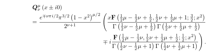
28: 14.23 Values on the Cut

… ►In terms of the hypergeometric function $𝐅$ (§14.3(i)) ►

14.23.3 $${𝑸}_{\nu }^{\mu }\left(x\pm \mathrm{i}0\right)=\frac{{\mathrm{e}}^{\mp \nu \pi \mathrm{i}/2}{\pi }^{3/2}{\left(1-x^2\right)}^{\mu /2}}{2^{\nu +1}}\left(\frac{x𝐅(\frac{1}{2}\mu -\frac{1}{2}\nu +\frac{1}{2},\frac{1}{2}\nu +\frac{1}{2}\mu +1;\frac{3}{2};x^2)}{\mathrm{\Gamma }\left(\frac{1}{2}\nu -\frac{1}{2}\mu +\frac{1}{2}\right)\mathrm{\Gamma }\left(\frac{1}{2}\nu +\frac{1}{2}\mu +\frac{1}{2}\right)}\mp \mathrm{i}\frac{𝐅(\frac{1}{2}\mu -\frac{1}{2}\nu ,\frac{1}{2}\nu +\frac{1}{2}\mu +\frac{1}{2};\frac{1}{2};x^2)}{\mathrm{\Gamma }\left(\frac{1}{2}\nu -\frac{1}{2}\mu +1\right)\mathrm{\Gamma }\left(\frac{1}{2}\nu +\frac{1}{2}\mu +1\right)}\right).$$

ⓘ

Symbols:

$\mathrm{\Gamma }\left(z\right)$: gamma function, ${𝑸}_{\nu }^{\mu }\left(z\right)$: Olver’s associated Legendre function, $\pi$: the ratio of the circumference of a circle to its diameter, $\mathrm{e}$: base of natural logarithm, $\mathrm{i}$: imaginary unit, $𝐅(a,b;c;z)$ or $𝐅(\genfrac{}{}{0pt}{}{a,b}{c};z)$: $={}_2{}^{}𝐅_1^{}(a,b;c;z)$ Olver’s hypergeometric function, $x$: real variable, $\mu$: general order and $\nu$: general degree

Referenced by:

§14.23

Permalink:

http://dlmf.nist.gov/14.23.E3

Encodings:

pMML, png, TeX

See also:

Annotations for §14.23 and Ch.14

…

29: 2.1 Definitions and Elementary Properties

… ►Then $\{{\varphi }_s(x)\}$ is an asymptotic sequence or scale. Suppose also that $f(x)$ and $f_s(x)$ satisfy …Then $\sum f_s(x)$ is a generalized asymptotic expansion of $f(x)$ with respect to the scale $\{{\varphi }_s(x)\}$. …

30: 14.1 Special Notation

… ► ►►►

$x$, $y$, $\tau$	real variables.
…
$𝐅(a,b;c;z)$	Olver’s scaled hypergeometric function: $F(a,b;c;z)/\mathrm{\Gamma }\left(c\right)$.

…