roots

SearchAdvancedHelp

(0.001 seconds)

11—20 of 83 matching pages

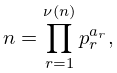
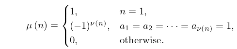
11: 27.2 Functions

… ►

27.2.1 $$n=\prod _{r=1}^{\nu \left(n\right)}{p}_r^{a_r},$$

ⓘ

Symbols:

$\nu \left(n\right)$: number of distinct primes dividing a number, $n$: positive integer, $p,p_1,\mathrm{\dots }$: prime numbers and $a$: primitive root

Referenced by:

§27.2(i), §27.3

Permalink:

http://dlmf.nist.gov/27.2.E1

Encodings:

pMML, png, TeX

See also:

Annotations for §27.2(i), §27.2 and Ch.27

… ►

27.2.8 $$a^{\varphi \left(n\right)}\equiv 1(modn),$$

ⓘ

Symbols:

$\varphi \left(n\right)$: Euler’s totient, $\equiv$: modular equivalence, $n$: positive integer and $a$: primitive root

A&S Ref:

24.3.2 II.B

Referenced by:

§27.16, §27.8

Permalink:

http://dlmf.nist.gov/27.2.E8

Encodings:

pMML, png, TeX

See also:

Annotations for §27.2(i), §27.2 and Ch.27

►and if $\varphi \left(n\right)$ is the smallest positive integer $f$ such that $a^f\equiv 1(modn)$, then $a$ is a primitive root mod $n$. … ►

27.2.12

ⓘ

Defines:

$\mu \left(n\right)$: Möbius function

Symbols:

$\nu \left(n\right)$: number of distinct primes dividing a number, $n$: positive integer and $a$: primitive root

A&S Ref:

24.3.1 I.A

Permalink:

http://dlmf.nist.gov/27.2.E12

Encodings:

pMML, png, TeX

See also:

Annotations for §27.2(i), §27.2 and Ch.27

… ►

27.2.13

ⓘ

Defines:

$\lambda \left(n\right)$: Liouville’s function

Symbols:

$\nu \left(n\right)$: number of distinct primes dividing a number, $n$: positive integer and $a$: primitive root

Permalink:

http://dlmf.nist.gov/27.2.E13

Encodings:

pMML, png, TeX

See also:

Annotations for §27.2(i), §27.2 and Ch.27

…

12: 18.37 Classical OP’s in Two or More Variables

… ►

§18.37(iii) OP’s Associated with Root Systems

►Orthogonal polynomials associated with root systems are certain systems of trigonometric polynomials in several variables, symmetric under a certain finite group (Weyl group), and orthogonal on a torus. …In several variables they occur, for $q=1$, as Jack polynomials and also as Jacobi polynomials associated with root systems; see Macdonald (1995, Chapter VI, §10), Stanley (1989), Kuznetsov and Sahi (2006, Part 1), Heckman (1991). For general $q$ they occur as Macdonald polynomials for root system $A_n$ , as Macdonald polynomials for general root systems, and as Macdonald–Koornwinder polynomials; see Macdonald (1995, Chapter VI), Macdonald (2000, 2003), Koornwinder (1992).

13: 19.31 Probability Distributions

… ► $R_G(x,y,z)$ and $R_F(x,y,z)$ occur as the expectation values, relative to a normal probability distribution in ${ℝ}^2$ or ${ℝ}^3$, of the square root or reciprocal square root of a quadratic form. …

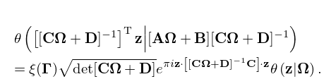
14: 21.5 Modular Transformations

… ►

21.5.4 $$\theta \left({\left[{[𝐂𝛀+𝐃]}^{-1}\right]}^{\mathrm{T}}𝐳\right|[𝐀𝛀+𝐁]{[𝐂𝛀+𝐃]}^{-1})=\xi (𝚪)\sqrt{det[𝐂𝛀+𝐃]}{\mathrm{e}}^{\pi \mathrm{i}𝐳\cdot \left[{[𝐂𝛀+𝐃]}^{-1}𝐂\right]\cdot 𝐳}\theta \left(𝐳\right|𝛀).$$

ⓘ

Symbols:

$\theta \left(𝐳\right|𝛀)$: Riemann theta function, $\pi$: the ratio of the circumference of a circle to its diameter, $det$: determinant, $\mathrm{e}$: base of natural logarithm, $\mathrm{i}$: imaginary unit, ${𝐀}^{\mathrm{T}}$: transpose of matrix, $𝛀$: a Riemann matrix, Matrix $𝚪$ and $\xi (𝚪)$: eighth root of unity

Referenced by:

§21.5(i)

Permalink:

http://dlmf.nist.gov/21.5.E4

Encodings:

pMML, png, TeX

See also:

Annotations for §21.5(i), §21.5 and Ch.21

►Here $\xi (𝚪)$ is an eighth root of unity, that is, ${(\xi (𝚪))}^8=1$. For general $𝚪$, it is difficult to decide which root needs to be used. … ►where the square root assumes its principal value. …

15: 23.5 Special Lattices

… ►In this case the lattice roots $e_1$, $e_2$, and $e_3$ are real and distinct. … ►The lattice root $e_1$ is real, and $e_3=\overline{e_2}$, with $\mathrm{\Im }{e}_2>0$. …As a function of $\mathrm{\Im }{e}_3$ the root $e_1$ is increasing. … ►and the lattice roots and invariants are given by ►

23.5.7 $$e_1={\mathrm{e}}^{2\pi \mathrm{i}/3}{e}_3={\mathrm{e}}^{-2\pi \mathrm{i}/3}{e}_2=\frac{{\left(\mathrm{\Gamma }\left(\frac{1}{3}\right)\right)}^6}{2^{14/3}{\pi }^2{\omega }_1^2},$$

ⓘ

Symbols:

$\mathrm{\Gamma }\left(z\right)$: gamma function, $e_j$: Weierstrass lattice roots, $\pi$: the ratio of the circumference of a circle to its diameter, $\mathrm{e}$: base of natural logarithm, $\mathrm{i}$: imaginary unit, $𝕃$: lattice and ${\omega }_1$, ${\omega }_3$, ${\omega }_2=-{\omega }_1-{\omega }_3$: lattice generators

Referenced by:

§23.22(ii)

Permalink:

http://dlmf.nist.gov/23.5.E7

Encodings:

pMML, png, TeX

See also:

Annotations for §23.5(v), §23.5 and Ch.23

…

16: 23.22 Methods of Computation

… ►

In the general case, given by $cd\ne 0$, we compute the roots $\alpha$, $\beta$, $\gamma$, say, of the cubic equation $4t^3-ct-d=0$; see §1.11(iii). These roots are necessarily distinct and represent $e_1$, $e_2$, $e_3$ in some order.

If $c$ and $d$ are real, and the discriminant is positive, that is $c^3-27d^2>0$, then $e_1$, $e_2$, $e_3$ can be identified via (23.5.1), and $k^2$, $k_{}^{\prime }{}_{}{}^2$ obtained from (23.6.16).

If , or $c$ and $d$ are not both real, then we label $\alpha$, $\beta$, $\gamma$ so that the triangle with vertices $\alpha$, $\beta$, $\gamma$ is positively oriented and $[\alpha ,\gamma ]$ is its longest side (chosen arbitrarily if there is more than one). In particular, if $\alpha$, $\beta$, $\gamma$ are collinear, then we label them so that $\beta$ is on the line segment $(\alpha ,\gamma )$. In consequence, $k^2=(\beta -\gamma )/(\alpha -\gamma )$, $k_{}^{\prime }{}_{}{}^2=(\alpha -\beta )/(\alpha -\gamma )$ satisfy $\mathrm{\Im }{k}^2\ge 0\ge \mathrm{\Im }k_{}^{\prime }{}_{}{}^2$ (with strict inequality unless $\alpha$, $\beta$, $\gamma$ are collinear); also $|k^2|$, $|k_{}^{\prime }{}_{}{}^2|\le 1$.

Finally, on taking the principal square roots of $k^2$ and $k_{}^{\prime }{}_{}{}^2$ we obtain values for $k$ and $k^{\prime }$ that lie in the 1st and 4th quadrants, respectively, and $2{\omega }_1$, $2{\omega }_3$ are given by

23.22.1 $$2{\omega }_{1}M(1,k^{\prime })=-2\mathrm{i}{\omega }_{3}M(1,k)=\frac{\pi }{3}\sqrt{\frac{c(2+k^{2}k_{}^{\prime }{}_{}{}^2)(k_{}^{\prime }{}_{}{}^2-k^2)}{d(1-k^{2}k_{}^{\prime }{}_{}{}^2)}},$$

ⓘ

Symbols:

$M(a,g)$: arithmetic-geometric mean, $\pi$: the ratio of the circumference of a circle to its diameter, $\mathrm{i}$: imaginary unit, ${\omega }_1$, ${\omega }_3$, ${\omega }_2=-{\omega }_1-{\omega }_3$: lattice generators, $k$: modulus and $k^{\prime }$: complementary modulus

Proof sketch:

Combine (23.6.16), (23.6.17), (22.20.6), (23.3.5)–(23.3.7), and use analytical continuation.

Referenced by:

§23.22(ii)

Permalink:

http://dlmf.nist.gov/23.22.E1

Encodings:

pMML, png, TeX

See also:

Annotations for §23.22(ii), §23.22(ii), §23.22 and Ch.23

where $M$ denotes the arithmetic-geometric mean (see §§19.8(i) and 22.20(ii)). This process yields 2 possible pairs ($2{\omega }_1$, $2{\omega }_3$), corresponding to the 2 possible choices of the square root.

…

17: 23.6 Relations to Other Functions

… ►In this subsection $2{\omega }_1$, $2{\omega }_3$ are any pair of generators of the lattice $𝕃$, and the lattice roots $e_1$, $e_2$, $e_3$ are given by (23.3.9). … ►

23.6.2 $$e_1=\frac{{\pi }^2}{12{\omega }_1^2}\left({\theta }_2^4(0,q)+2{\theta }_4^4(0,q)\right),$$

ⓘ

Symbols:

${\theta }_j(z,q)$: theta function, $e_j$: Weierstrass lattice roots, $\pi$: the ratio of the circumference of a circle to its diameter, $𝕃$: lattice, $q$: nome and ${\omega }_1$, ${\omega }_3$, ${\omega }_2=-{\omega }_1-{\omega }_3$: lattice generators

A&S Ref:

18.10.12, 18.10.13, 18.10.14, and 18.10.9, 18.10.10, 18.10.11

Referenced by:

§23.22(ii), §23.22(i), §23.6(i), §23.6(ii)

Permalink:

http://dlmf.nist.gov/23.6.E2

Encodings:

pMML, png, TeX

See also:

Annotations for §23.6(i), §23.6 and Ch.23

►

23.6.3 $$e_2=\frac{{\pi }^2}{12{\omega }_1^2}\left({\theta }_2^4(0,q)-{\theta }_4^4(0,q)\right),$$

ⓘ

Symbols:

${\theta }_j(z,q)$: theta function, $e_j$: Weierstrass lattice roots, $\pi$: the ratio of the circumference of a circle to its diameter, $𝕃$: lattice, $q$: nome and ${\omega }_1$, ${\omega }_3$, ${\omega }_2=-{\omega }_1-{\omega }_3$: lattice generators

A&S Ref:

18.10.12, 18.10.13, 18.10.14, and 18.10.9, 18.10.10, 18.10.11

Permalink:

http://dlmf.nist.gov/23.6.E3

Encodings:

pMML, png, TeX

See also:

Annotations for §23.6(i), §23.6 and Ch.23

… ►

23.6.20 $$e_3=-\frac{K^2}{3{\omega }_1^2}(1+k^2).$$

ⓘ

Symbols:

$e_j$: Weierstrass lattice roots, $K\left(k\right)$: Legendre’s complete elliptic integral of the first kind, $𝕃$: lattice, ${\omega }_1$, ${\omega }_3$, ${\omega }_2=-{\omega }_1-{\omega }_3$: lattice generators and $k$: modulus

A&S Ref:

18.9.3

Referenced by:

§23.6(ii)

Permalink:

http://dlmf.nist.gov/23.6.E20

Encodings:

pMML, png, TeX

See also:

Annotations for §23.6(ii), §23.6 and Ch.23

… ►Then $z=\mathrm{\wp }\left(w\right)$, where the value of $w$ depends on the choice of path and determination of the square root; see McKean and Moll (1999, pp. 87–88 and §2.5). …

18: 20.12 Mathematical Applications

… ►For an application of a generalization in affine root systems see Macdonald (1972). …

19: 27.21 Tables

… ►8 gives examples of primitive roots of all primes $\le 9973$; Table 24. …

20: 36.5 Stokes Sets

… ►where $x_{\pm }$ are the two smallest positive roots of the equation … ►For $\left|Y\right|>Y_1$ the second sheet is generated by a second solution of (36.5.6)–(36.5.9), and for it is generated by the roots of the polynomial equation … ►Here $u$ is the root of the equation … ►where $u$ is the root of the equation … ►where $u$ is the positive root of the equation …