roots of constants

SearchAdvancedHelp

(0.002 seconds)

1—10 of 42 matching pages

1: 1.11 Zeros of Polynomials

… ►

§1.11(iv) Roots of Unity and of Other Constants

…

2: 23.22 Methods of Computation

… ►

In the general case, given by $cd\ne 0$, we compute the roots $\alpha$, $\beta$, $\gamma$, say, of the cubic equation $4t^3-ct-d=0$; see §1.11(iii). These roots are necessarily distinct and represent $e_1$, $e_2$, $e_3$ in some order.

If $c$ and $d$ are real, and the discriminant is positive, that is $c^3-27d^2>0$, then $e_1$, $e_2$, $e_3$ can be identified via (23.5.1), and $k^2$, $k_{}^{\prime }{}_{}{}^2$ obtained from (23.6.16).

If , or $c$ and $d$ are not both real, then we label $\alpha$, $\beta$, $\gamma$ so that the triangle with vertices $\alpha$, $\beta$, $\gamma$ is positively oriented and $[\alpha ,\gamma ]$ is its longest side (chosen arbitrarily if there is more than one). In particular, if $\alpha$, $\beta$, $\gamma$ are collinear, then we label them so that $\beta$ is on the line segment $(\alpha ,\gamma )$. In consequence, $k^2=(\beta -\gamma )/(\alpha -\gamma )$, $k_{}^{\prime }{}_{}{}^2=(\alpha -\beta )/(\alpha -\gamma )$ satisfy $\mathrm{\Im }{k}^2\ge 0\ge \mathrm{\Im }k_{}^{\prime }{}_{}{}^2$ (with strict inequality unless $\alpha$, $\beta$, $\gamma$ are collinear); also $|k^2|$, $|k_{}^{\prime }{}_{}{}^2|\le 1$.

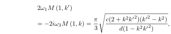
Finally, on taking the principal square roots of $k^2$ and $k_{}^{\prime }{}_{}{}^2$ we obtain values for $k$ and $k^{\prime }$ that lie in the 1st and 4th quadrants, respectively, and $2{\omega }_1$, $2{\omega }_3$ are given by

23.22.1 $$2{\omega }_{1}M(1,k^{\prime })=-2\mathrm{i}{\omega }_{3}M(1,k)=\frac{\pi }{3}\sqrt{\frac{c(2+k^{2}k_{}^{\prime }{}_{}{}^2)(k_{}^{\prime }{}_{}{}^2-k^2)}{d(1-k^{2}k_{}^{\prime }{}_{}{}^2)}},$$

ⓘ

Symbols:

$M(a,g)$: arithmetic-geometric mean, $\pi$: the ratio of the circumference of a circle to its diameter, $\mathrm{i}$: imaginary unit, ${\omega }_1$, ${\omega }_3$, ${\omega }_2=-{\omega }_1-{\omega }_3$: lattice generators, $k$: modulus and $k^{\prime }$: complementary modulus

Proof sketch:

Combine (23.6.16), (23.6.17), (22.20.6), (23.3.5)–(23.3.7), and use analytical continuation.

Referenced by:

§23.22(ii)

Permalink:

http://dlmf.nist.gov/23.22.E1

Encodings:

pMML, png, TeX

See also:

Annotations for §23.22(ii), §23.22(ii), §23.22 and Ch.23

where $M$ denotes the arithmetic-geometric mean (see §§19.8(i) and 22.20(ii)). This process yields 2 possible pairs ($2{\omega }_1$, $2{\omega }_3$), corresponding to the 2 possible choices of the square root.

…

3: 31.2 Differential Equations

… ►

31.2.10 $$w(\xi )={\left(\mathrm{\wp }\left(\xi \right)-e_3\right)}^{(1-2\gamma )/4}{\left(\mathrm{\wp }\left(\xi \right)-e_2\right)}^{(1-2\delta )/4}{\left(\mathrm{\wp }\left(\xi \right)-e_1\right)}^{(1-2ϵ)/4}W(\xi ),$$

ⓘ

Symbols:

$\mathrm{\wp }\left(z\right)$ (= $\mathrm{\wp }\left(z|𝕃\right)$ = $\mathrm{\wp }(z;g_2,g_3)$): Weierstrass $\mathrm{\wp }$-function, $e_j$: Weierstrass lattice roots, $\gamma$: real or complex parameter, $\delta$: real or complex parameter, $ϵ$: real or complex parameter, $𝕃$: lattice and $W(\xi )$: solution

Permalink:

http://dlmf.nist.gov/31.2.E10

Encodings:

pMML, png, TeX

See also:

Annotations for §31.2(iv), §31.2(iv), §31.2 and Ch.31

…

4: 21.5 Modular Transformations

… ►

21.5.4 $$\theta \left({\left[{[𝐂𝛀+𝐃]}^{-1}\right]}^{\mathrm{T}}𝐳\right|[𝐀𝛀+𝐁]{[𝐂𝛀+𝐃]}^{-1})=\xi (𝚪)\sqrt{det[𝐂𝛀+𝐃]}{\mathrm{e}}^{\pi \mathrm{i}𝐳\cdot \left[{[𝐂𝛀+𝐃]}^{-1}𝐂\right]\cdot 𝐳}\theta \left(𝐳\right|𝛀).$$

ⓘ

Symbols:

$\theta \left(𝐳\right|𝛀)$: Riemann theta function, $\pi$: the ratio of the circumference of a circle to its diameter, $det$: determinant, $\mathrm{e}$: base of natural logarithm, $\mathrm{i}$: imaginary unit, ${𝐀}^{\mathrm{T}}$: transpose of matrix, $𝛀$: a Riemann matrix, Matrix $𝚪$ and $\xi (𝚪)$: eighth root of unity

Referenced by:

§21.5(i)

Permalink:

http://dlmf.nist.gov/21.5.E4

Encodings:

pMML, png, TeX

See also:

Annotations for §21.5(i), §21.5 and Ch.21

►Here $\xi (𝚪)$ is an eighth root of unity, that is, ${(\xi (𝚪))}^8=1$. For general $𝚪$, it is difficult to decide which root needs to be used. …

5: 2.9 Difference Equations

… ►

2.9.9 $$w_j(n)\sim {\rho }^n\exp \left({(-1)}^j\kappa \sqrt{n}\right)n^{\alpha }\sum _{s=0}^{\mathrm{\infty }}{(-1)}^{js}\frac{c_s}{n^{s/2}},$$

ⓘ

Symbols:

$\sim$: Poincaré asymptotic expansion, $\exp z$: exponential function, $\rho$: roots, $\kappa$ , $c$: constant and $w_j(n)$: solutions

Permalink:

http://dlmf.nist.gov/2.9.E9

Encodings:

pMML, png, TeX

See also:

Annotations for §2.9(ii), §2.9 and Ch.2

… ►

2.9.13 $$w_2(n)\sim {\rho }^n{n}^{{\alpha }_2}\sum _{\begin{array}{c}s=0\\ s\ne {\alpha }_2-{\alpha }_1\end{array}}^{\mathrm{\infty }}\frac{b_s}{n^s}+c{w}_1(n)\ln n,$$ $n\to \mathrm{\infty }$.

ⓘ

Symbols:

$\sim$: Poincaré asymptotic expansion, $\ln z$: principal branch of logarithm function, $\rho$: roots, $b_s$: coefficients, $c$: constant and $w_j(n)$: solutions

Permalink:

http://dlmf.nist.gov/2.9.E13

Encodings:

pMML, png, TeX

See also:

Annotations for §2.9(ii), §2.9 and Ch.2

…

6: 2.7 Differential Equations

… ►

2.7.12 $$a_{s,1}\sim \frac{{\mathrm{\Lambda }}_1}{{({\lambda }_1-{\lambda }_2)}^s}\sum _{j=0}^{\mathrm{\infty }}{a}_{j,2}{({\lambda }_1-{\lambda }_2)}^j\mathrm{\Gamma }\left(s+{\mu }_2-{\mu }_1-j\right),$$

ⓘ

Symbols:

$\mathrm{\Gamma }\left(z\right)$: gamma function, $\sim$: Poincaré asymptotic expansion, $a_{s,j}$: coefficients, ${\lambda }_j$: roots, ${\mu }_j$: quantities and ${\mathrm{\Lambda }}_j$: constants

Referenced by:

§2.11(v), §2.7(ii)

Permalink:

http://dlmf.nist.gov/2.7.E12

Encodings:

pMML, png, TeX

See also:

Annotations for §2.7(ii), §2.7 and Ch.2

►

2.7.13 $$a_{s,2}\sim \frac{{\mathrm{\Lambda }}_2}{{({\lambda }_2-{\lambda }_1)}^s}\sum _{j=0}^{\mathrm{\infty }}{a}_{j,1}{({\lambda }_2-{\lambda }_1)}^j\mathrm{\Gamma }\left(s+{\mu }_1-{\mu }_2-j\right),$$

ⓘ

Symbols:

$\mathrm{\Gamma }\left(z\right)$: gamma function, $\sim$: Poincaré asymptotic expansion, $a_{s,j}$: coefficients, ${\lambda }_j$: roots, ${\mu }_j$: quantities and ${\mathrm{\Lambda }}_j$: constants

Referenced by:

§2.11(v), §2.7(ii)

Permalink:

http://dlmf.nist.gov/2.7.E13

Encodings:

pMML, png, TeX

See also:

Annotations for §2.7(ii), §2.7 and Ch.2

… ►

2.7.15 $$-\frac{3}{2}\pi +\delta \le \mathrm{ph}\left(({\lambda }_2-{\lambda }_1)z\right)\le \frac{3}{2}\pi -\delta ,$$ $j=1$,

ⓘ

Symbols:

$\pi$: the ratio of the circumference of a circle to its diameter, $\mathrm{ph}$: phase, ${\lambda }_j$: roots and $\delta$: arbitrary small positive constant

Referenced by:

§2.7(ii)

Permalink:

http://dlmf.nist.gov/2.7.E15

Encodings:

pMML, png, TeX

See also:

Annotations for §2.7(ii), §2.7 and Ch.2

►

2.7.16 $$-\frac{1}{2}\pi +\delta \le \mathrm{ph}\left(({\lambda }_2-{\lambda }_1)z\right)\le \frac{5}{2}\pi -\delta ,$$ $j=2$,

ⓘ

Symbols:

$\pi$: the ratio of the circumference of a circle to its diameter, $\mathrm{ph}$: phase, ${\lambda }_j$: roots and $\delta$: arbitrary small positive constant

Referenced by:

§2.7(ii)

Permalink:

http://dlmf.nist.gov/2.7.E16

Encodings:

pMML, png, TeX

See also:

Annotations for §2.7(ii), §2.7 and Ch.2

…

7: 21.7 Riemann Surfaces

… ►Either branch of the square roots may be chosen, as long as the branch is consistent across $\mathrm{\Gamma }$. …

8: 28.31 Equations of Whittaker–Hill and Ince

… ►and constant values of $A,B,k$, and $c$, is called the Equation of Whittaker–Hill. … ►When , we substitute … ►

28.31.4 $$w_{e,s}(z)=\sum _{\mathrm{\ell }=0}^{\mathrm{\infty }}{A}_{2\mathrm{\ell }+s}\cos (2\mathrm{\ell }+s)z,$$ $s=0,1$,

ⓘ

Symbols:

$\cos z$: cosine function, $z$: complex variable, $w(z)$: Mathieu’s equation solution and $A$: constant

Referenced by:

§28.31(ii)

Permalink:

http://dlmf.nist.gov/28.31.E4

Encodings:

pMML, png, TeX

See also:

Annotations for §28.31(ii), §28.31 and Ch.28

►

28.31.5 $$w_{o,s}(z)=\sum _{\mathrm{\ell }=0}^{\mathrm{\infty }}{B}_{2\mathrm{\ell }+s}\sin (2\mathrm{\ell }+s)z,$$ $s=1,2$,

ⓘ

Symbols:

$\sin z$: sine function, $z$: complex variable, $w(z)$: Mathieu’s equation solution and $B$: constant

Referenced by:

§28.31(ii)

Permalink:

http://dlmf.nist.gov/28.31.E5

Encodings:

pMML, png, TeX

See also:

Annotations for §28.31(ii), §28.31 and Ch.28

…

9: 23.5 Special Lattices

… ►

23.5.7 $$e_1={\mathrm{e}}^{2\pi \mathrm{i}/3}{e}_3={\mathrm{e}}^{-2\pi \mathrm{i}/3}{e}_2=\frac{{\left(\mathrm{\Gamma }\left(\frac{1}{3}\right)\right)}^6}{2^{14/3}{\pi }^2{\omega }_1^2},$$

ⓘ

Symbols:

$\mathrm{\Gamma }\left(z\right)$: gamma function, $e_j$: Weierstrass lattice roots, $\pi$: the ratio of the circumference of a circle to its diameter, $\mathrm{e}$: base of natural logarithm, $\mathrm{i}$: imaginary unit, $𝕃$: lattice and ${\omega }_1$, ${\omega }_3$, ${\omega }_2=-{\omega }_1-{\omega }_3$: lattice generators

Referenced by:

§23.22(ii)

Permalink:

http://dlmf.nist.gov/23.5.E7

Encodings:

pMML, png, TeX

See also:

Annotations for §23.5(v), §23.5 and Ch.23

…

10: 2.8 Differential Equations with a Parameter

… ►

2.8.34 $$\mathrm{env}{J}_{\nu }(x)=\mathrm{env}{Y}_{\nu }(x)={\left(J_{\nu }^2(x)+Y_{\nu }^2(x)\right)}^{1/2},$$ .

ⓘ

Symbols:

$J_{\nu }\left(z\right)$: Bessel function of the first kind, $Y_{\nu }\left(z\right)$: Bessel function of the second kind, $\mathrm{env}{J}_{\nu }\left(x\right)$: envelope of Bessel function $J_{\nu }\left(x\right)$ , $\mathrm{env}{Y}_{\nu }\left(x\right)$: envelope of Bessel function $Y_{\nu }\left(x\right)$ , $\nu$: real nonnegative constant and $X_{\nu }$: smallest positive root

Permalink:

http://dlmf.nist.gov/2.8.E34

Encodings:

pMML, png, TeX

See also:

Annotations for §2.8(iv), §2.8 and Ch.2

…