reparametrization of integration paths
(0.004 seconds)
1—10 of 171 matching pages
1: 1.6 Vectors and Vector-Valued Functions
…
►
§1.6(iv) Path and Line Integrals
… ►The path integral of a continuous function is …A path , , is a reparametrization of , , if and with differentiable and monotonic. If and , then the reparametrization is called orientation-preserving, and …If and , then the reparametrization is orientation-reversing and …2: 31.18 Methods of Computation
…
►Independent solutions of (31.2.1) can be computed in the neighborhoods of singularities from their Fuchs–Frobenius expansions (§31.3), and elsewhere by numerical integration of (31.2.1).
…Care needs to be taken to choose integration paths in such a way that the wanted solution is growing in magnitude along the path at least as rapidly as all other solutions (§3.7(ii)).
…
3: 9.17 Methods of Computation
…
►A comprehensive and powerful approach is to integrate the defining differential equation (9.2.1) by direct numerical methods.
As described in §3.7(ii), to ensure stability the integration path must be chosen in such a way that as we proceed along it the wanted solution grows at least as fast as all other solutions of the differential equation.
…On the remaining rays, given by and , integration can proceed in either direction.
…
►In the case of the Scorer functions, integration of the differential equation (9.12.1) is more difficult than (9.2.1), because in some regions stable directions of integration do not exist.
…
►In the first method the integration path for the contour integral (9.5.4) is deformed to coincide with paths of steepest descent (§2.4(iv)).
…
4: 31.9 Orthogonality
…
►The integration path begins at , encircles once in the positive sense, followed by once in the positive sense, and so on, returning finally to .
The integration path is called a Pochhammer double-loop
contour (compare Figure 5.12.3).
The branches of the many-valued functions are continuous on the path, and assume their principal values at the beginning.
…
►and the integration paths
, are Pochhammer double-loop contours encircling distinct pairs of singularities , , .
…
►For bi-orthogonal relations for path-multiplicative solutions see Schmidt (1979, §2.2).
…
5: 11.13 Methods of Computation
…
►A comprehensive approach is to integrate the defining inhomogeneous differential equations (11.2.7) and (11.2.9) numerically, using methods described in §3.7.
To insure stability the integration path must be chosen so that as we proceed along it the wanted solution grows in magnitude at least as rapidly as the complementary solutions.
…
►Then from the limiting forms for small argument (§§11.2(i), 10.7(i), 10.30(i)), limiting forms for large argument (§§11.6(i), 10.7(ii), 10.30(ii)), and the connection formulas (11.2.5) and (11.2.6), it is seen that and can be computed in a stable manner by integrating forwards, that is, from the origin toward infinity.
The solution needs to be integrated backwards for small , and either forwards or backwards for large depending whether or not exceeds .
For both forward and backward integration are unstable, and boundary-value methods are required (§3.7(iii)).
…
6: 8.6 Integral Representations
…
►
takes its principal value where the path intersects the positive real axis, and is continuous elsewhere on the path.
…where the integration path passes above or below the pole at , according as upper or lower signs are taken.
…
►In (8.6.10)–(8.6.12), is a real constant and the path of integration is indented (if necessary) so that in the case of (8.6.10) it separates the poles of the gamma function from the pole at , in the case of (8.6.11) it is to the right of all poles, and in the case of (8.6.12) it separates the poles of the gamma function from the poles at .
…
7: 15.19 Methods of Computation
…
►A comprehensive and powerful approach is to integrate the hypergeometric differential equation (15.10.1) by direct numerical methods.
As noted in §3.7(ii), the integration path should be chosen so that the wanted solution grows in magnitude at least as fast as all other solutions.
However, since the growth near the singularities of the differential equation is algebraic rather than exponential, the resulting instabilities in the numerical integration might be tolerable in some cases.
…
8: 26.2 Basic Definitions
…
►
Lattice Path
►A lattice path is a directed path on the plane integer lattice . …For an example see Figure 26.9.2. ►A k-dimensional lattice path is a directed path composed of segments that connect vertices in so that each segment increases one coordinate by exactly one unit. …9: 2.4 Contour Integrals
…
►If is analytic in a sector containing , then the region of validity may be increased by rotation of the integration paths.
…
►Then by integration by parts the integral
…
►Cases in which are usually handled by deforming the integration path in such a way that the minimum of is attained at a saddle point or at an endpoint.
…However, for the purpose of simply deriving the asymptotic expansions the use of steepest descent paths is not essential.
…
►Suppose that on the integration path
there are two simple zeros of that coincide for a certain value of .
…
