regularization

SearchAdvancedHelp

(0.002 seconds)

1—10 of 53 matching pages

1: 33.8 Continued Fractions

… ►

33.8.1 $$\frac{F_{\mathrm{\ell }}^{\prime }}{F_{\mathrm{\ell }}}=S_{\mathrm{\ell }+1}-\frac{R_{\mathrm{\ell }+1}^2}{T_{\mathrm{\ell }+1}-}\frac{R_{\mathrm{\ell }+2}^2}{T_{\mathrm{\ell }+2}-}\mathrm{\cdots }.$$

ⓘ

Symbols:

$F_{\mathrm{\ell }}(\eta ,\rho )$: regular Coulomb radial function, $\mathrm{\ell }$: nonnegative integer, $R_{\mathrm{\ell }}$: factor, $S_{\mathrm{\ell }}$: factor and $T_{\mathrm{\ell }}$: factor

Referenced by:

§33.8, §33.8

Permalink:

http://dlmf.nist.gov/33.8.E1

Encodings:

pMML, png, TeX

See also:

Annotations for §33.8 and Ch.33

… ►If we denote $u=F_{\mathrm{\ell }}^{\prime }/F_{\mathrm{\ell }}$ and $p+\mathrm{i}q=H_{\mathrm{\ell }}^{+}{}_{}{}^{\prime }/H_{\mathrm{\ell }}^{+}$, then ►

$F_{\mathrm{\ell }}=\pm {(q^{-1}{(u-p)}^2+q)}^{-1/2},$

►

$F_{\mathrm{\ell }}^{\prime }=u{F}_{\mathrm{\ell }},$

►

$G_{\mathrm{\ell }}=q^{-1}(u-p)F_{\mathrm{\ell }},$

…

2: 33.3 Graphics

… ►

§33.3(i) Line Graphs of the Coulomb Radial Functions $F_{\mathrm{\ell }}(\eta ,\rho )$ and $G_{\mathrm{\ell }}(\eta ,\rho )$

►

►►

Figure 33.3.1: $F_{\mathrm{\ell }}(\eta ,\rho )$, $G_{\mathrm{\ell }}(\eta ,\rho )$ with $\mathrm{\ell }=0$, $\eta =-2$. Magnify

►

►►

Figure 33.3.2: $F_{\mathrm{\ell }}(\eta ,\rho )$, $G_{\mathrm{\ell }}(\eta ,\rho )$ with $\mathrm{\ell }=0$, $\eta =0$. Magnify

►

►►

Figure 33.3.3: $F_{\mathrm{\ell }}(\eta ,\rho )$, $G_{\mathrm{\ell }}(\eta ,\rho )$ with $\mathrm{\ell }=0$, $\eta =2$. … Magnify

… ►

§33.3(ii) Surfaces of the Coulomb Radial Functions $F_0(\eta ,\rho )$ and $G_0(\eta ,\rho )$

…

3: 25.17 Physical Applications

… ►Quantum field theory often encounters formally divergent sums that need to be evaluated by a process of regularization: for example, the energy of the electromagnetic vacuum in a confined space (Casimir–Polder effect). It has been found possible to perform such regularizations by equating the divergent sums to zeta functions and associated functions (Elizalde (1995)).

4: 33.23 Methods of Computation

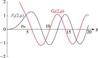
… ►The power-series expansions of §§33.6 and 33.19 converge for all finite values of the radii $\rho$ and $r$, respectively, and may be used to compute the regular and irregular solutions. … ►Thus the regular solutions can be computed from the power-series expansions (§§33.6, 33.19) for small values of the radii and then integrated in the direction of increasing values of the radii. … ►This implies decreasing $\mathrm{\ell }$ for the regular solutions and increasing $\mathrm{\ell }$ for the irregular solutions of §§33.2(iii) and 33.14(iii). … ►§33.8 supplies continued fractions for $F_{\mathrm{\ell }}^{\prime }/F_{\mathrm{\ell }}$ and $H_{\mathrm{\ell }}^{\pm }{}_{}{}^{\prime }/H_{\mathrm{\ell }}^{\pm }$. Combined with the Wronskians (33.2.12), the values of $F_{\mathrm{\ell }}$, $G_{\mathrm{\ell }}$, and their derivatives can be extracted. …

5: 33.2 Definitions and Basic Properties

… ►

§33.2(i) Coulomb Wave Equation

… ►This differential equation has a regular singularity at $\rho =0$ with indices $\mathrm{\ell }+1$ and $-\mathrm{\ell }$, and an irregular singularity of rank 1 at $\rho =\mathrm{\infty }$ (§§2.7(i), 2.7(ii)). … ►

§33.2(ii) Regular Solution $F_{\mathrm{\ell }}(\eta ,\rho )$

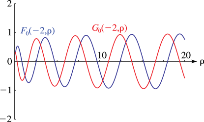
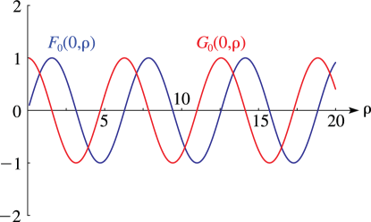
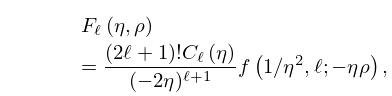
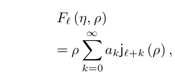
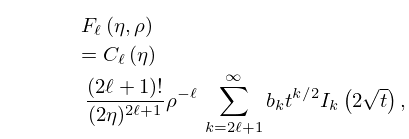
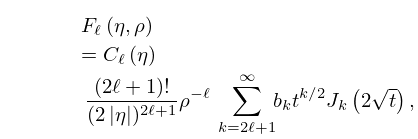
►The function $F_{\mathrm{\ell }}(\eta ,\rho )$ is recessive (§2.7(iii)) at $\rho =0$, and is defined by … ► $F_{\mathrm{\ell }}(\eta ,\rho )$ is a real and analytic function of $\rho$ on the open interval , and also an analytic function of $\eta$ when . …

6: 33.5 Limiting Forms for Small $\rho$, Small $|\eta |$, or Large $\mathrm{\ell }$

… ►

$F_{\mathrm{\ell }}(\eta ,\rho )\sim C_{\mathrm{\ell }}\left(\eta \right){\rho }^{\mathrm{\ell }+1},$

►

$F_{\mathrm{\ell }}^{\prime }(\eta ,\rho )\sim (\mathrm{\ell }+1)C_{\mathrm{\ell }}\left(\eta \right){\rho }^{\mathrm{\ell }}.$

… ►

$F_{\mathrm{\ell }}(0,\rho )=\rho {𝗃}_{\mathrm{\ell }}\left(\rho \right),$

… ►

$F_0(0,\rho )=\sin \rho ,$

… ►

$F_{\mathrm{\ell }}(\eta ,\rho )\sim C_{\mathrm{\ell }}\left(\eta \right){\rho }^{\mathrm{\ell }+1},$

…

7: 33.24 Tables

… ►

Abramowitz and Stegun (1964, Chapter 14) tabulates $F_0(\eta ,\rho )$, $G_0(\eta ,\rho )$, $F_0^{\prime }(\eta ,\rho )$, and $G_0^{\prime }(\eta ,\rho )$ for $\eta =0.5(.5)20$ and $\rho =1(1)20$, 5S; $C_0\left(\eta \right)$ for $\eta =0(.05)3$, 6S.

…

8: 33.10 Limiting Forms for Large $\rho$ or Large $\left|\eta \right|$

… ►

$$F_{\mathrm{\ell }}(\eta ,\rho )=\sin \left({\theta }_{\mathrm{\ell }}(\eta ,\rho )\right)+o\left(1\right),$$

… ►

$F_{\mathrm{\ell }}(\eta ,\rho )\sim {\displaystyle \frac{(2\mathrm{\ell }+1)!C_{\mathrm{\ell }}\left(\eta \right)}{{(2\eta )}^{\mathrm{\ell }+1}}}{(2\eta \rho )}^{1/2}{I}_{2\mathrm{\ell }+1}\left({(8\eta \rho )}^{1/2}\right),$

… ►

$$F_0(\eta ,\rho )\sim {\mathrm{e}}^{-\pi \eta }{(\pi \rho )}^{1/2}{I}_1\left({(8\eta \rho )}^{1/2}\right),$$

… ►

$$F_0^{\prime }(\eta ,\rho )\sim {\mathrm{e}}^{-\pi \eta }{(2\pi \eta )}^{1/2}{I}_0\left({(8\eta \rho )}^{1/2}\right),$$

… ►

$$F_0(\eta ,\rho )={(\pi \rho )}^{1/2}{J}_1\left({(-8\eta \rho )}^{1/2}\right)+o\left({\left|\eta \right|}^{-1/4}\right),$$

…

9: 33.16 Connection Formulas

… ►

§33.16(i) $F_{\mathrm{\ell }}$ and $G_{\mathrm{\ell }}$ in Terms of $f$ and $h$

►

33.16.1 $$F_{\mathrm{\ell }}(\eta ,\rho )=\frac{(2\mathrm{\ell }+1)!C_{\mathrm{\ell }}\left(\eta \right)}{{(-2\eta )}^{\mathrm{\ell }+1}}f(1/{\eta }^2,\mathrm{\ell };-\eta \rho ),$$

ⓘ

Symbols:

$C_{\mathrm{\ell }}\left(\eta \right)$: normalizing constant for Coulomb radial functions, $f(ϵ,\mathrm{\ell };r)$: regular Coulomb function, $!$: factorial (as in $n!$), $F_{\mathrm{\ell }}(\eta ,\rho )$: regular Coulomb radial function, $\mathrm{\ell }$: nonnegative integer, $\rho$: nonnegative real variable and $\eta$: real parameter

Referenced by:

§33.18

Permalink:

http://dlmf.nist.gov/33.16.E1

Encodings:

pMML, png, TeX

See also:

Annotations for §33.16(i), §33.16 and Ch.33

… ►

§33.16(ii) $f$ and $h$ in Terms of $F_{\mathrm{\ell }}$ and $G_{\mathrm{\ell }}$ when $ϵ>0$

… ►

33.16.4 $$f(ϵ,\mathrm{\ell };r)={\left(\frac{2}{\pi \tau }\frac{1-{\mathrm{e}}^{-2\pi /\tau }}{A(ϵ,\mathrm{\ell })}\right)}^{1/2}{F}_{\mathrm{\ell }}(-1/\tau ,\tau r),$$

ⓘ

Symbols:

$f(ϵ,\mathrm{\ell };r)$: regular Coulomb function, $\pi$: the ratio of the circumference of a circle to its diameter, $\mathrm{e}$: base of natural logarithm, $F_{\mathrm{\ell }}(\eta ,\rho )$: regular Coulomb radial function, $\mathrm{\ell }$: nonnegative integer, $r$: real variable, $ϵ$: real parameter, $A(ϵ,\mathrm{\ell })$: function and $\tau$: parameter

Referenced by:

§33.16(iv), item 1

Permalink:

http://dlmf.nist.gov/33.16.E4

Encodings:

pMML, png, TeX

See also:

Annotations for §33.16(ii), §33.16 and Ch.33

… ►

§33.16(iv) $s$ and $c$ in Terms of $F_{\mathrm{\ell }}$ and $G_{\mathrm{\ell }}$ when $ϵ>0$

…

10: 33.9 Expansions in Series of Bessel Functions

… ►

33.9.1 $$F_{\mathrm{\ell }}(\eta ,\rho )=\rho \sum _{k=0}^{\mathrm{\infty }}{a}_k{𝗃}_{\mathrm{\ell }+k}\left(\rho \right),$$

ⓘ

Symbols:

$F_{\mathrm{\ell }}(\eta ,\rho )$: regular Coulomb radial function, ${𝗃}_n\left(z\right)$: spherical Bessel function of the first kind, $k$: nonnegative integer, $\mathrm{\ell }$: nonnegative integer, $\rho$: nonnegative real variable, $\eta$: real parameter and $a_k$: coefficients

A&S Ref:

14.4.5

Referenced by:

§33.9(i), §33.9(i)

Permalink:

http://dlmf.nist.gov/33.9.E1

Encodings:

pMML, png, TeX

See also:

Annotations for §33.9(i), §33.9 and Ch.33

… ►

33.9.3 $$F_{\mathrm{\ell }}(\eta ,\rho )=C_{\mathrm{\ell }}\left(\eta \right)\frac{(2\mathrm{\ell }+1)!}{{(2\eta )}^{2\mathrm{\ell }+1}}{\rho }^{-\mathrm{\ell }}\sum _{k=2\mathrm{\ell }+1}^{\mathrm{\infty }}{b}_k{t}^{k/2}{I}_k\left(2\sqrt{t}\right),$$ $\eta >0$,

ⓘ

Symbols:

$C_{\mathrm{\ell }}\left(\eta \right)$: normalizing constant for Coulomb radial functions, $!$: factorial (as in $n!$), $I_{\nu }\left(z\right)$: modified Bessel function of the first kind, $F_{\mathrm{\ell }}(\eta ,\rho )$: regular Coulomb radial function, $k$: nonnegative integer, $\mathrm{\ell }$: nonnegative integer, $\rho$: nonnegative real variable, $\eta$: real parameter, $t$: parameter and $b_k$: coefficient

A&S Ref:

14.4.1

Referenced by:

§33.9(ii), §33.9(ii)

Permalink:

http://dlmf.nist.gov/33.9.E3

Encodings:

pMML, png, TeX

See also:

Annotations for §33.9(ii), §33.9 and Ch.33

►

33.9.4 $$F_{\mathrm{\ell }}(\eta ,\rho )=C_{\mathrm{\ell }}\left(\eta \right)\frac{(2\mathrm{\ell }+1)!}{{(2\left|\eta \right|)}^{2\mathrm{\ell }+1}}{\rho }^{-\mathrm{\ell }}\sum _{k=2\mathrm{\ell }+1}^{\mathrm{\infty }}{b}_k{t}^{k/2}{J}_k\left(2\sqrt{t}\right),$$ .

ⓘ

Symbols:

$J_{\nu }\left(z\right)$: Bessel function of the first kind, $C_{\mathrm{\ell }}\left(\eta \right)$: normalizing constant for Coulomb radial functions, $!$: factorial (as in $n!$), $F_{\mathrm{\ell }}(\eta ,\rho )$: regular Coulomb radial function, $k$: nonnegative integer, $\mathrm{\ell }$: nonnegative integer, $\rho$: nonnegative real variable, $\eta$: real parameter, $t$: parameter and $b_k$: coefficient

Referenced by:

§33.9(ii), §33.9(ii)

Permalink:

http://dlmf.nist.gov/33.9.E4

Encodings:

pMML, png, TeX

See also:

Annotations for §33.9(ii), §33.9 and Ch.33

…