regular solutions

SearchAdvancedHelp

(0.002 seconds)

11—20 of 28 matching pages

11: 15.11 Riemann’s Differential Equation

… ►The importance of (15.10.1) is that any homogeneous linear differential equation of the second order with at most three distinct singularities, all regular, in the extended plane can be transformed into (15.10.1). The most general form is given by … ►denotes the set of solutions of (15.10.1). ►

§15.11(ii) Transformation Formulas

… ►The reduction of a general homogeneous linear differential equation of the second order with at most three regular singularities to the hypergeometric differential equation is given by …

12: 31.12 Confluent Forms of Heun’s Equation

… ►Confluent forms of Heun’s differential equation (31.2.1) arise when two or more of the regular singularities merge to form an irregular singularity. … ►This has regular singularities at $z=0$ and $1$, and an irregular singularity of rank 1 at $z=\mathrm{\infty }$. ►Mathieu functions (Chapter 28), spheroidal wave functions (Chapter 30), and Coulomb spheroidal functions (§30.12) are special cases of solutions of the confluent Heun equation. … ►This has a regular singularity at $z=0$, and an irregular singularity at $\mathrm{\infty }$ of rank $2$. … ►This has one singularity, an irregular singularity of rank $3$ at $z=\mathrm{\infty }$. …

13: 13.2 Definitions and Basic Properties

… ►This equation has a regular singularity at the origin with indices $0$ and $1-b$, and an irregular singularity at infinity of rank one. …In effect, the regular singularities of the hypergeometric differential equation at $b$ and $\mathrm{\infty }$ coalesce into an irregular singularity at $\mathrm{\infty }$. ►

Standard Solutions

… ►

§13.2(v) Numerically Satisfactory Solutions

… ► …

14: Bibliography

… ►

Computation of the regular confluent hypergeometric function. The Mathematica Journal 5 (4), pp. 74–76.

ⓘ

External Links:

ISSN 1047-5974, FullText

Referenced by:

§13.32(iii).

Encodings:

BibTeX

►

Asymptotics of solutions of the generalized sine-Gordon equation, the third Painlevé equation and the d’Alembert equation. Dokl. Akad. Nauk SSSR 280 (2), pp. 265–268 (Russian).

ⓘ

Notes:

English translation: Soviet Math. Dokl. 31(1985), no. 1, pp. 45–47

External Links:

ISSN 0002-3264, MathReview (M. S. Agranovich), ZentralBlatt

Referenced by:

§32.11(iv).

Encodings:

BibTeX

… ►

Regular and irregular Coulomb wave functions expressed in terms of Bessel-Clifford functions. J. Math. Physics 33, pp. 111–116.

ⓘ

External Links:

MathReview (E. Weber), ZentralBlatt

Referenced by:

§33.9(ii).

Encodings:

BibTeX

… ►

Rational solutions of Painlevé equations. Stud. Appl. Math. 61 (1), pp. 31–53.

ⓘ

External Links:

ISSN 0022-2526, MathReview (H. Hochstadt), ZentralBlatt

Referenced by:

§32.10(ii), §32.8(i), §32.8(v).

Encodings:

BibTeX

… ►

Perturbation solutions of the ellipsoidal wave equation. Quart. J. Math. Oxford Ser. (2) 7, pp. 161–174.

ⓘ

External Links:

ISSN 0033-5606, Document, MathReview (A. Erdélyi), ZentralBlatt

Referenced by:

§29.11.

Encodings:

BibTeX

…

15: 13.14 Definitions and Basic Properties

… ►It has a regular singularity at the origin with indices $\frac{1}{2}\pm \mu$, and an irregular singularity at infinity of rank one. ►

Standard Solutions

►Standard solutions are: … ►

§13.14(v) Numerically Satisfactory Solutions

►Fundamental pairs of solutions of (13.14.1) that are numerically satisfactory (§2.7(iv)) in the neighborhood of infinity are …

16: 10.2 Definitions

… ►This differential equation has a regular singularity at $z=0$ with indices $\pm \nu$, and an irregular singularity at $z=\mathrm{\infty }$ of rank $1$; compare §§2.7(i) and 2.7(ii). ►

§10.2(ii) Standard Solutions

… ►This solution of (10.2.1) is an analytic function of $z\in ℂ$, except for a branch point at $z=0$ when $\nu$ is not an integer. … ►Each solution has a branch point at $z=0$ for all $\nu \in ℂ$. … ►

§10.2(iii) Numerically Satisfactory Pairs of Solutions

…

17: 2.7 Differential Equations

… ►All solutions are analytic at an ordinary point, and their Taylor-series expansions are found by equating coefficients. …

18: 10.47 Definitions and Basic Properties

… ►Equations (10.47.1) and (10.47.2) each have a regular singularity at $z=0$ with indices $n$, $-n-1$, and an irregular singularity at $z=\mathrm{\infty }$ of rank $1$; compare §§2.7(i)–2.7(ii). … ►

§10.47(ii) Standard Solutions

… ►

§10.47(iii) Numerically Satisfactory Pairs of Solutions

►For (10.47.1) numerically satisfactory pairs of solutions are given by Table 10.2.1 with the symbols $J$, $Y$, $H$, and $\nu$ replaced by $𝗃$, $𝗒$, $𝗁$, and $n$, respectively. ►For (10.47.2) numerically satisfactory pairs of solutions are ${𝗂}_n^{(1)}\left(z\right)$ and ${𝗄}_n\left(z\right)$ in the right half of the $z$-plane, and ${𝗂}_n^{(1)}\left(z\right)$ and ${𝗄}_n\left(-z\right)$ in the left half of the $z$-plane. …

19: 30.2 Differential Equations

… ►

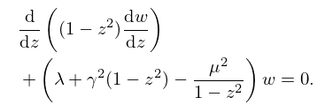
30.2.1 $$\frac{d}{dz}\left((1-z^2)\frac{dw}{dz}\right)+\left(\lambda +{\gamma }^2(1-z^2)-\frac{{\mu }^2}{1-z^2}\right)w=0.$$

ⓘ

Symbols:

$\frac{df}{dx}$: derivative of $f$ with respect to $x$ , $z$: complex variable, $w$: solution to DE, $\lambda$: real parameter, ${\gamma }^2$: real parameter and $\mu$: real parameter

Referenced by:

§30.11(i), §30.12, §30.12, §30.13(iv), §30.14(iv), §30.16(ii), §30.2(ii), §30.2(iii), §30.3(i), §30.4(i), §30.5, §30.6, §30.6

Permalink:

http://dlmf.nist.gov/30.2.E1

Encodings:

pMML, png, TeX

See also:

Annotations for §30.2(i), §30.2 and Ch.30

►This equation has regular singularities at $z=\pm 1$ with exponents $\pm \frac{1}{2}\mu$ and an irregular singularity of rank 1 at $z=\mathrm{\infty }$ (if $\gamma \ne 0$). … ►

30.2.4 $$({\zeta }^2-{\gamma }^2)\frac{d^{2}w}{{d\zeta }^2}+2\zeta \frac{dw}{d\zeta }+\left({\zeta }^2-\lambda -{\gamma }^2-\frac{{\gamma }^2{\mu }^2}{{\zeta }^2-{\gamma }^2}\right)w=0.$$

ⓘ

Symbols:

$\frac{df}{dx}$: derivative of $f$ with respect to $x$ , $w$: solution to DE, $\lambda$: real parameter, ${\gamma }^2$: real parameter, $\mu$: real parameter and $\zeta$: parameter

Referenced by:

§30.2(iii)

Permalink:

http://dlmf.nist.gov/30.2.E4

Encodings:

pMML, png, TeX

See also:

Annotations for §30.2(ii), §30.2 and Ch.30

…

20: 29.2 Differential Equations

… ►

29.2.1 $$\frac{d^{2}w}{{dz}^2}+(h-\nu (\nu +1)k^2{\mathrm{sn}}^2(z,k))w=0,$$

ⓘ

Symbols:

$\mathrm{sn}(z,k)$: Jacobian elliptic function, $\frac{df}{dx}$: derivative of $f$ with respect to $x$ , $z$: complex variable, $h$: real parameter, $k$: real parameter, $\nu$: real parameter and $w(z)$: solution

Referenced by:

§29.10, §29.11, §29.12(i), §29.17(i), §29.17(ii), §29.17(iii), §29.18(i), §29.2(i), §29.20(i), §29.3(i), §29.7(ii), §29.8, §29.9

Permalink:

http://dlmf.nist.gov/29.2.E1

Encodings:

pMML, png, TeX

See also:

Annotations for §29.2(i), §29.2 and Ch.29

… ►This equation has regular singularities at the points $2pK+(2q+1)\mathrm{i}{K}^{\prime }$, where $p,q\in \mathbb{Z}$, and $K$, $K^{\prime }$ are the complete elliptic integrals of the first kind with moduli $k$, $k^{\prime }(={(1-k^2)}^{1/2})$, respectively; see §19.2(ii). In general, at each singularity each solution of (29.2.1) has a branch point (§2.7(i)). …