real%20and%20imaginary%20parts
(0.006 seconds)
1—10 of 19 matching pages
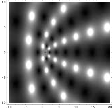
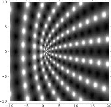
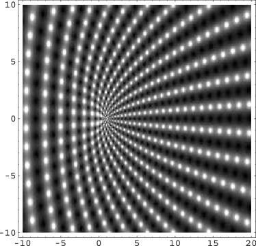
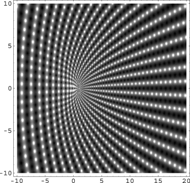
1: 22.3 Graphics
 ►
►
 ►
►
 ►
►
 ►
►
2: 10.75 Tables
Zhang and Jin (1996, pp. 185–195) tabulates , , , , , , 5, 10, 25, 50, 100, 9S; , , , , , , , 8S; real and imaginary parts of , , , , , , , , 8S.
Zhang and Jin (1996, pp. 240–250) tabulates , , , , , , 9S; , , , , , 10, 30, 50, 100, , , , , , , 5, 10, 50, 8S; real and imaginary parts of , , , , , 20(10)50, 100, , , 8S.
Zhang and Jin (1996, pp. 296–305) tabulates , , , , , , , , , 50, 100, , 5, 10, 25, 50, 100, 8S; , , , (Riccati–Bessel functions and their derivatives), , 50, 100, , 5, 10, 25, 50, 100, 8S; real and imaginary parts of , , , , , , , , , 20(10)50, 100, , , 8S. (For the notation replace by , , , , respectively.)
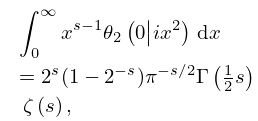
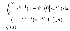
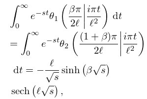
3: 20.10 Integrals
4: 6.19 Tables
Abramowitz and Stegun (1964, Chapter 5) includes the real and imaginary parts of , , , 6D; , , , 6D; , , , 6D.
Zhang and Jin (1996, pp. 690–692) includes the real and imaginary parts of , , , 8S.
5: Software Index
| Open Source | With Book | Commercial | |||||||||||||||||||||||
| … | |||||||||||||||||||||||||
| 10.77(vi) Bessel Functions–Imaginary Order and Real Argument | ✓ | ✓ | ✓ | ✓ | ✓ | ✓ | ✓ | ||||||||||||||||||
| … | |||||||||||||||||||||||||
| 16.27(ii) Real Arguments | ✓ | ✓ | ✓ | ✓ | a | ✓ | ✓ | ✓ | ✓ | ||||||||||||||||
| … | |||||||||||||||||||||||||
| 20 Theta Functions | |||||||||||||||||||||||||
| … | |||||||||||||||||||||||||
| 22.22(ii) Real Argument | ✓ | ✓ | ✓ | ✓ | ✓ | ✓ | ✓ | ✓ | ✓ | ✓ | ✓ | ✓ | ✓ | ✓ | ✓ | ✓ | |||||||||
| … | |||||||||||||||||||||||||
Such software ranges from a collection of reusable software parts (e.g., a library) to fully functional interactive computing environments with an associated computing language. Such software is usually professionally developed, tested, and maintained to high standards. It is available for purchase, often with accompanying updates and consulting support.
6: 9.18 Tables
Zhang and Jin (1996, p. 337) tabulates , , , for to 8S and for to 9D.
Woodward and Woodward (1946) tabulates the real and imaginary parts of , , , for , . Precision is 4D.
Harvard University (1945) tabulates the real and imaginary parts of , , , for , , , with interval 0.1 in and . Precision is 8D. Here , .
Corless et al. (1992) gives the real and imaginary parts of for ; 14S.
Nosova and Tumarkin (1965) tabulates , , , for ; 7D. Also included are the real and imaginary parts of and , where and ; 6-7D.
7: 25.12 Polylogarithms
8: 7.23 Tables
Zhang and Jin (1996, pp. 638, 640–641) includes the real and imaginary parts of , , , 7D and 8D, respectively; the real and imaginary parts of , , , 8D, together with the corresponding modulus and phase to 8D and 6D (degrees), respectively.
