radial

SearchAdvancedHelp

(0.000 seconds)

1—10 of 42 matching pages

1: 30.11 Radial Spheroidal Wave Functions

§30.11 Radial Spheroidal Wave Functions

►

§30.11(i) Definitions

… ►

Connection Formulas

… ►

§30.11(ii) Graphics

… ►

§30.11(iv) Wronskian

…

2: 28.20 Definitions and Basic Properties

… ►

§28.20(iv) Radial Mathieu Functions ${\mathrm{Mc}}_n^{(j)}$, ${\mathrm{Ms}}_n^{(j)}$

… ►

28.20.15 $${\mathrm{Mc}}_n^{(j)}(z,h)={\mathrm{M}}_n^{(j)}(z,h),$$ $n=0,1,\mathrm{\dots }$,

ⓘ

Defines:

${\mathrm{Mc}}_n^{(j)}(z,h)$: radial Mathieu function

Symbols:

${\mathrm{M}}_{\nu }^{(j)}(z,h)$: modified Mathieu function, $h$: parameter, $n$: integer, $j$: integer and $z$: complex variable

Referenced by:

§28.20(vii)

Permalink:

http://dlmf.nist.gov/28.20.E15

Encodings:

pMML, png, TeX

See also:

Annotations for §28.20(iv), §28.20 and Ch.28

►

28.20.16 $${\mathrm{Ms}}_n^{(j)}(z,h)={(-1)}^n{\mathrm{M}}_{-n}^{(j)}(z,h),$$ $n=1,2,\mathrm{\dots }$.

ⓘ

Defines:

${\mathrm{Ms}}_n^{(j)}(z,h)$: radial Mathieu function

Symbols:

${\mathrm{M}}_{\nu }^{(j)}(z,h)$: modified Mathieu function, $h$: parameter, $n$: integer, $j$: integer and $z$: complex variable

Referenced by:

§28.20(vii)

Permalink:

http://dlmf.nist.gov/28.20.E16

Encodings:

pMML, png, TeX

See also:

Annotations for §28.20(iv), §28.20 and Ch.28

… ►

§28.20(vii) Shift of Variable

… ►And for the corresponding identities for the radial functions use (28.20.15) and (28.20.16).

3: 30.17 Tables

§30.17 Tables

… ►

Hanish et al. (1970) gives ${\lambda }_n^m\left({\gamma }^2\right)$ and $S_n^{m(j)}(z,\gamma )$, $j=1,2$, and their first derivatives, for $0\le m\le 2$, $m\le n\le m+49$, $-1600\le {\gamma }^2\le 1600$. The range of $z$ is given by $1\le z\le 10$ if ${\gamma }^2>0$, or $z=-\mathrm{i}\xi$, $0\le \xi \le 2$ if . Precision is 18S.

►

EraŠevskaja et al. (1973, 1976) gives $S^{m(j)}(\mathrm{i}y,-\mathrm{i}c)$, $S^{m(j)}(z,\gamma )$ and their first derivatives for $j=1,2$, $0.5\le c\le 8$, $y=0,0.5,1,1.5$, $0.5\le \gamma \le 8$, $z=1.01,1.1,1.4,1.8$. Precision is 15S.

…

4: 33.3 Graphics

… ►

§33.3(i) Line Graphs of the Coulomb Radial Functions $F_{\mathrm{\ell }}(\eta ,\rho )$ and $G_{\mathrm{\ell }}(\eta ,\rho )$

… ►

►►

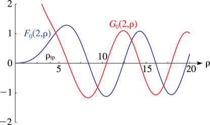
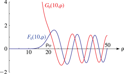
Figure 33.3.3: $F_{\mathrm{\ell }}(\eta ,\rho )$, $G_{\mathrm{\ell }}(\eta ,\rho )$ with $\mathrm{\ell }=0$, $\eta =2$. The turning point is at ${\rho }_{\mathrm{tp}}(2,0)=4$. Magnify

►

►►

Figure 33.3.4: $F_{\mathrm{\ell }}(\eta ,\rho )$, $G_{\mathrm{\ell }}(\eta ,\rho )$ with $\mathrm{\ell }=0$, $\eta =10$. The turning point is at ${\rho }_{\mathrm{tp}}(10,0)=20$. Magnify

… ►

►►

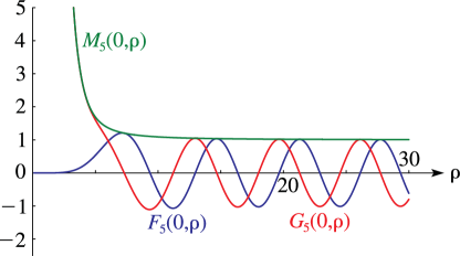
Figure 33.3.6: $F_{\mathrm{\ell }}(\eta ,\rho )$, $G_{\mathrm{\ell }}(\eta ,\rho )$, and $M_{\mathrm{\ell }}(\eta ,\rho )$ with $\mathrm{\ell }=5$, $\eta =0$. The turning point is at ${\rho }_{\mathrm{tp}}(0,5)=\sqrt{30}$ (as in Figure 33.3.5). Magnify

►

§33.3(ii) Surfaces of the Coulomb Radial Functions $F_0(\eta ,\rho )$ and $G_0(\eta ,\rho )$

…

5: 28.21 Graphics

… ►

Radial Mathieu Functions: Surfaces

… ►

►

►

Figure 28.21.6: ${\mathrm{Ms}}_1^{(2)}(x,h)$ for $0.2\le h\le 2$, $0\le x\le 2$. Magnify 3D Help

6: 30.1 Special Notation

… ►The main functions treated in this chapter are the eigenvalues ${\lambda }_n^m\left({\gamma }^2\right)$ and the spheroidal wave functions ${\mathrm{𝖯𝗌}}_n^m(x,{\gamma }^2)$, ${\mathrm{𝖰𝗌}}_n^m(x,{\gamma }^2)$, ${\mathrm{𝑃𝑠}}_n^m(z,{\gamma }^2)$, ${\mathrm{𝑄𝑠}}_n^m(z,{\gamma }^2)$, and $S_n^{m(j)}(z,\gamma )$, $j=1,2,3,4$. … ►Flammer (1957) and Abramowitz and Stegun (1964) use ${\lambda }_{mn}(\gamma )$ for ${\lambda }_n^m\left({\gamma }^2\right)+{\gamma }^2$, $R_{mn}^{(j)}(\gamma ,z)$ for $S_n^{m(j)}(z,\gamma )$, and …

7: 30.18 Software

… ►

SWF4: $S_n^{m(j)}(z,\gamma )$, $j=1,2$.

…

8: 33.5 Limiting Forms for Small $\rho$, Small $|\eta |$, or Large $\mathrm{\ell }$

… ►

33.5.6 $$C_{\mathrm{\ell }}\left(0\right)=\frac{2^{\mathrm{\ell }}\mathrm{\ell }!}{(2\mathrm{\ell }+1)!}=\frac{1}{(2\mathrm{\ell }+1)!!}.$$

ⓘ

Symbols:

$C_{\mathrm{\ell }}\left(\eta \right)$: normalizing constant for Coulomb radial functions, $!!$: double factorial, $!$: factorial (as in $n!$) and $\mathrm{\ell }$: nonnegative integer

Permalink:

http://dlmf.nist.gov/33.5.E6

Encodings:

pMML, png, TeX

See also:

Annotations for §33.5(ii), §33.5 and Ch.33

… ►

33.5.9 $$C_{\mathrm{\ell }}\left(\eta \right)\sim \frac{{\mathrm{e}}^{-\pi \eta /2}}{(2\mathrm{\ell }+1)!!}\sim {\mathrm{e}}^{-\pi \eta /2}\frac{{\mathrm{e}}^{\mathrm{\ell }}}{\sqrt{2}{(2\mathrm{\ell })}^{\mathrm{\ell }+1}}.$$

ⓘ

Symbols:

$C_{\mathrm{\ell }}\left(\eta \right)$: normalizing constant for Coulomb radial functions, $\sim$: asymptotic equality, $\pi$: the ratio of the circumference of a circle to its diameter, $!!$: double factorial, $\mathrm{e}$: base of natural logarithm, $\mathrm{\ell }$: nonnegative integer and $\eta$: real parameter

Referenced by:

§33.23(iv), §33.5(iv)

Permalink:

http://dlmf.nist.gov/33.5.E9

Encodings:

pMML, png, TeX

See also:

Annotations for §33.5(iv), §33.5 and Ch.33

9: 33.23 Methods of Computation

… ►Use of extended-precision arithmetic increases the radial range that yields accurate results, but eventually other methods must be employed, for example, the asymptotic expansions of §§33.11 and 33.21. … ►Inside the turning points, that is, when , there can be a loss of precision by a factor of approximately ${|G_{\mathrm{\ell }}|}^2$. … ►Curtis (1964a, §10) describes the use of series, radial integration, and other methods to generate the tables listed in §33.24. … ►WKBJ approximations (§2.7(iii)) for $\rho >{\rho }_{\mathrm{tp}}(\eta ,\mathrm{\ell })$ are presented in Hull and Breit (1959) and Seaton and Peach (1962: in Eq. … ►Hull and Breit (1959) and Barnett (1981b) give WKBJ approximations for $F_0$ and $G_0$ in the region inside the turning point: .

10: 30.14 Wave Equation in Oblate Spheroidal Coordinates

… ►

30.14.8 $$w_1(\xi )=a_1{S}_n^{m(1)}(\mathrm{i}\xi ,\gamma )+b_1{S}_n^{m(2)}(\mathrm{i}\xi ,\gamma ).$$

ⓘ

Symbols:

$\mathrm{i}$: imaginary unit, $S_n^{m(j)}(z,\gamma )$: radial spheroidal wave function, $m$: nonnegative integer, $n\ge m$: integer degree, $b_j$: coefficients, $a_j$: coefficients, $\xi$: oblate spheroidal coordinate, $w_j$: solution to DE and ${\gamma }^2={\kappa }^2{c}^2$: parameter

Referenced by:

§30.14(v)

Permalink:

http://dlmf.nist.gov/30.14.E8

Encodings:

pMML, png, TeX

See also:

Annotations for §30.14(iv), §30.14 and Ch.30

… ►

§30.14(v) The Interior Dirichlet Problem for Oblate Ellipsoids

… ►

30.14.9 $$S_n^{m(1)}(\mathrm{i}{\xi }_0,\gamma )=0.$$

ⓘ

Symbols:

$\mathrm{i}$: imaginary unit, $S_n^{m(j)}(z,\gamma )$: radial spheroidal wave function, $m$: nonnegative integer, $n\ge m$: integer degree, $\xi$: oblate spheroidal coordinate and ${\gamma }^2$: real parameter

Permalink:

http://dlmf.nist.gov/30.14.E9

Encodings:

pMML, png, TeX

See also:

Annotations for §30.14(v), §30.14 and Ch.30

…