q-cosine function

SearchAdvancedHelp

(0.003 seconds)

10 matching pages

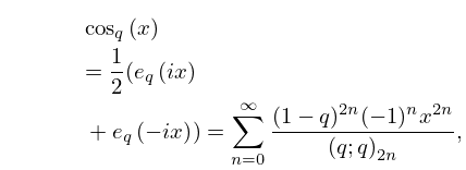
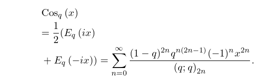
1: 17.3 $q$-Elementary and $q$-Special Functions

… ►

$q$-Cosine Functions

►

17.3.5 $${\cos }_q\left(x\right)=\frac{1}{2}(e_q\left(\mathrm{i}x\right)+e_q\left(-\mathrm{i}x\right))=\sum _{n=0}^{\mathrm{\infty }}\frac{{(1-q)}^{2n}{(-1)}^n{x}^{2n}}{{(q;q)}_{2n}},$$

ⓘ

Defines:

${\cos }_q\left(x\right)$: $q$-cosine function

Symbols:

$\mathrm{i}$: imaginary unit, ${(a;q)}_n$: $q$-Pochhammer symbol (or $q$-shifted factorial), $e_q\left(x\right)$: $q$-exponential function, $q$: complex base, $n$: nonnegative integer and $x$: real variable

Permalink:

http://dlmf.nist.gov/17.3.E5

Encodings:

pMML, png, TeX

See also:

Annotations for §17.3(i), §17.3(i), §17.3 and Ch.17

►

17.3.6 $${\mathrm{Cos}}_q\left(x\right)=\frac{1}{2}(E_q\left(\mathrm{i}x\right)+E_q\left(-\mathrm{i}x\right))=\sum _{n=0}^{\mathrm{\infty }}\frac{{(1-q)}^{2n}{q}^{n(2n-1)}{(-1)}^n{x}^{2n}}{{(q;q)}_{2n}}.$$

ⓘ

Defines:

${\mathrm{Cos}}_q\left(x\right)$: $q$-cosine function

Symbols:

$\mathrm{i}$: imaginary unit, $E_q\left(x\right)$: $q$-exponential function, ${(a;q)}_n$: $q$-Pochhammer symbol (or $q$-shifted factorial), $q$: complex base, $n$: nonnegative integer and $x$: real variable

Permalink:

http://dlmf.nist.gov/17.3.E6

Encodings:

pMML, png, TeX

See also:

Annotations for §17.3(i), §17.3(i), §17.3 and Ch.17

…

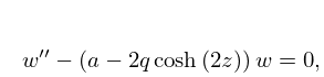
2: 28.2 Definitions and Basic Properties

… ►

28.2.1 $$w^{\prime \prime }+(a-2q\cos \left(2z\right))w=0.$$

ⓘ

Symbols:

$\cos z$: cosine function, $q=h^2$: parameter, $z$: complex variable, $a$: parameter and $w(z)$: Mathieu’s equation solution

A&S Ref:

20.3.1 20.1.1 (in slightly different form)

Referenced by:

§1.18(vii), Figure 28.17.1, Figure 28.17.1, §28.17, §28.17, §28.2(ii), §28.2(ii), §28.2(iii), §28.2(iv), §28.20(i), §28.29(i), §28.32(i), §28.32(i), 1st item, 2nd item, §28.33(iii), item (a), item (c), item (c), §28.5(i), §28.8(iv), §28.8(iv), §28.8(iv), §30.2(iii)

Permalink:

http://dlmf.nist.gov/28.2.E1

Encodings:

pMML, png, TeX

See also:

Annotations for §28.2(i), §28.2 and Ch.28

…

3: 28.20 Definitions and Basic Properties

… ►

28.20.1 $$w^{\prime \prime }-\left(a-2q\cosh \left(2z\right)\right)w=0,$$

ⓘ

Symbols:

$\cosh z$: hyperbolic cosine function, $q=h^2$: parameter, $z$: complex variable, $a$: parameter and $w(z)$: Mathieu’s equation solution

A&S Ref:

20.1.2 (in slightly different form) 20.8.6

Referenced by:

§28.20(iii), §28.32(i), 1st item, 2nd item, item (b), §28.8(iv), §28.8(iv)

Permalink:

http://dlmf.nist.gov/28.20.E1

Encodings:

pMML, png, TeX

See also:

Annotations for §28.20(i), §28.20 and Ch.28

…

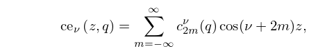
4: 28.14 Fourier Series

… ►

28.14.2 $${\mathrm{ce}}_{\nu }(z,q)=\sum _{m=-\mathrm{\infty }}^{\mathrm{\infty }}{c}_{2m}^{\nu }(q)\cos (\nu +2m)z,$$

ⓘ

Symbols:

${\mathrm{ce}}_n(z,q)$: Mathieu function, $\cos z$: cosine function, $m$: integer, $q=h^2$: parameter, $z$: complex variable, $\nu$: complex parameter and $c_{2m}(q)$: coefficients

Permalink:

http://dlmf.nist.gov/28.14.E2

Encodings:

pMML, png, TeX

See also:

Annotations for §28.14 and Ch.28

…

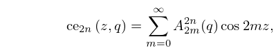
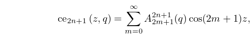
5: 28.4 Fourier Series

… ►

28.4.1 $${\mathrm{ce}}_{2n}(z,q)=\sum _{m=0}^{\mathrm{\infty }}{A}_{2m}^{2n}(q)\cos 2mz,$$

ⓘ

Symbols:

${\mathrm{ce}}_n(z,q)$: Mathieu function, $\cos z$: cosine function, $m$: integer, $q=h^2$: parameter, $n$: integer, $z$: complex variable and $A_m(q)$: Fourier coefficient

A&S Ref:

20.2.3 (in slightly different form) 20.2.4 (in slightly different form)

Permalink:

http://dlmf.nist.gov/28.4.E1

Encodings:

pMML, png, TeX

See also:

Annotations for §28.4(i), §28.4 and Ch.28

►

28.4.2 $${\mathrm{ce}}_{2n+1}(z,q)=\sum _{m=0}^{\mathrm{\infty }}{A}_{2m+1}^{2n+1}(q)\cos (2m+1)z,$$

ⓘ

Symbols:

${\mathrm{ce}}_n(z,q)$: Mathieu function, $\cos z$: cosine function, $m$: integer, $q=h^2$: parameter, $n$: integer, $z$: complex variable and $A_m(q)$: Fourier coefficient

Permalink:

http://dlmf.nist.gov/28.4.E2

Encodings:

pMML, png, TeX

See also:

Annotations for §28.4(i), §28.4 and Ch.28

…

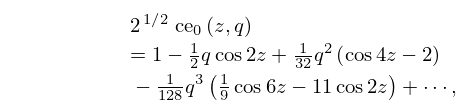
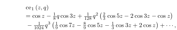
6: 28.6 Expansions for Small $q$

… ►

28.6.21 $$2^{1/2}{\mathrm{ce}}_0(z,q)=1-\frac{1}{2}q\cos 2z+\frac{1}{32}{q}^2\left(\cos 4z-2\right)-\frac{1}{128}{q}^3\left(\frac{1}{9}\cos 6z-11\cos 2z\right)+\mathrm{\cdots },$$

ⓘ

Symbols:

${\mathrm{ce}}_n(z,q)$: Mathieu function, $\cos z$: cosine function, $q=h^2$: parameter and $z$: complex variable

A&S Ref:

20.2.27

Referenced by:

§28.6(ii)

Permalink:

http://dlmf.nist.gov/28.6.E21

Encodings:

pMML, png, TeX

See also:

Annotations for §28.6(ii), §28.6 and Ch.28

►

28.6.22 $${\mathrm{ce}}_1(z,q)=\cos z-\frac{1}{8}q\cos 3z+\frac{1}{128}{q}^2\left(\frac{2}{3}\cos 5z-2\cos 3z-\cos z\right)-\frac{1}{1024}{q}^3\left(\frac{1}{9}\cos 7z-\frac{8}{9}\cos 5z-\frac{1}{3}\cos 3z+2\cos z\right)+\mathrm{\cdots },$$

ⓘ

Symbols:

${\mathrm{ce}}_n(z,q)$: Mathieu function, $\cos z$: cosine function, $q=h^2$: parameter and $z$: complex variable

Permalink:

http://dlmf.nist.gov/28.6.E22

Encodings:

pMML, png, TeX

See also:

Annotations for §28.6(ii), §28.6 and Ch.28

…

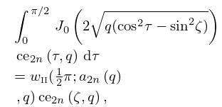
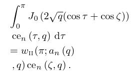
7: 28.10 Integral Equations

… ►

28.10.9 $${\int }_0^{\pi /2}{J}_0\left(2\sqrt{q({\cos }^2\tau -{\sin }^2\zeta )}\right){\mathrm{ce}}_{2n}(\tau ,q)d\tau =w_{\text{II}}(\frac{1}{2}\pi ;a_{2n}\left(q\right),q){\mathrm{ce}}_{2n}(\zeta ,q),$$

ⓘ

Symbols:

$J_{\nu }\left(z\right)$: Bessel function of the first kind, ${\mathrm{ce}}_n(z,q)$: Mathieu function, $a_n\left(q\right)$: eigenvalues of Mathieu equation, $\pi$: the ratio of the circumference of a circle to its diameter, $\cos z$: cosine function, $dx$: differential of $x$ , $\int$: integral, $\sin z$: sine function, $q=h^2$: parameter, $n$: integer and $w_{\text{II}}(z;a,q)$: fundamental solution

Permalink:

http://dlmf.nist.gov/28.10.E9

Encodings:

pMML, png, TeX

See also:

Annotations for §28.10(ii), §28.10 and Ch.28

►

28.10.10 $${\int }_0^{\pi }{J}_0\left(2\sqrt{q}(\cos \tau +\cos \zeta )\right){\mathrm{ce}}_n(\tau ,q)d\tau =w_{\text{II}}(\pi ;a_n\left(q\right),q){\mathrm{ce}}_n(\zeta ,q).$$

ⓘ

Symbols:

$J_{\nu }\left(z\right)$: Bessel function of the first kind, ${\mathrm{ce}}_n(z,q)$: Mathieu function, $a_n\left(q\right)$: eigenvalues of Mathieu equation, $\pi$: the ratio of the circumference of a circle to its diameter, $\cos z$: cosine function, $dx$: differential of $x$ , $\int$: integral, $q=h^2$: parameter, $n$: integer and $w_{\text{II}}(z;a,q)$: fundamental solution

Permalink:

http://dlmf.nist.gov/28.10.E10

Encodings:

pMML, png, TeX

See also:

Annotations for §28.10(ii), §28.10 and Ch.28

…

8: 28.32 Mathematical Applications

… ►

28.32.4 $$\frac{{\partial }^{2}K}{{\partial z}^2}-\frac{{\partial }^{2}K}{{\partial \zeta }^2}=2q\left(\cos \left(2z\right)-\cos \left(2\zeta \right)\right)K.$$

ⓘ

Symbols:

$\cos z$: cosine function, $\frac{\partial f}{\partial x}$: partial derivative of $f$ with respect to $x$ , $\partial x$: partial differential of $x$ , $q=h^2$: parameter, $z$: complex variable, $\zeta$: variable and $K(z,\zeta )$: solution

Permalink:

http://dlmf.nist.gov/28.32.E4

Encodings:

pMML, png, TeX

See also:

Annotations for §28.32(i), §28.32 and Ch.28

…

9: 28.9 Zeros

§28.9 Zeros

►For real $q$ each of the functions ${\mathrm{ce}}_{2n}(z,q)$, ${\mathrm{se}}_{2n+1}(z,q)$, ${\mathrm{ce}}_{2n+1}(z,q)$, and ${\mathrm{se}}_{2n+2}(z,q)$ has exactly $n$ zeros in . They are continuous in $q$. For $q\to \mathrm{\infty }$ the zeros of ${\mathrm{ce}}_{2n}(z,q)$ and ${\mathrm{se}}_{2n+1}(z,q)$ approach asymptotically the zeros of ${\mathrm{𝐻𝑒}}_{2n}\left(q^{1/4}(\pi -2z)\right)$, and the zeros of ${\mathrm{ce}}_{2n+1}(z,q)$ and ${\mathrm{se}}_{2n+2}(z,q)$ approach asymptotically the zeros of ${\mathrm{𝐻𝑒}}_{2n+1}\left(q^{1/4}(\pi -2z)\right)$. …Furthermore, for $q>0$ ${\mathrm{ce}}_m(z,q)$ and ${\mathrm{se}}_m(z,q)$ also have purely imaginary zeros that correspond uniquely to the purely imaginary $z$-zeros of $J_m\left(2\sqrt{q}\cos z\right)$ (§10.21(i)), and they are asymptotically equal as $q\to 0$ and $\left|\mathrm{\Im }z\right|\to \mathrm{\infty }$. …

10: 1.18 Linear Second Order Differential Operators and Eigenfunction Expansions

… ►The Fourier cosine and sine transform pairs (1.14.9) & (1.14.11) and (1.14.10) & (1.14.12) can be easily obtained from (1.18.57) as for $\nu =\pm \frac{1}{2}$ the Bessel functions reduce to the trigonometric functions, see (10.16.1). … ► … ►For example, replacing $2q\cos (2z)$ of (28.2.1) by $\lambda \cos (2\pi \alpha n+\theta )$, $n\in \mathbb{Z}$ gives an almost Mathieu equation which for appropriate $\alpha$ has such properties. … ►This dilatation transformation, which does require analyticity of $q(x)$ in (1.18.28), or an analytic approximation thereto, leaves the poles, corresponding to the discrete spectrum, invariant, as they are, as is the branch point, actual singularities of $⟨{\left(z-T\right)}^{-1}f,f⟩$. … ►Surprisingly, if on any interval on the real line, even if positive elsewhere, as long as ${\int }_{X}q(x)dx\le 0$, see Simon (1976, Theorem 2.5), then there will be at least one eigenfunction with a negative eigenvalue, with corresponding $L^2\left(X\right)$ eigenfunction. …