q-binomial%20series
(0.005 seconds)
1—10 of 336 matching pages
1: 17.5 Functions
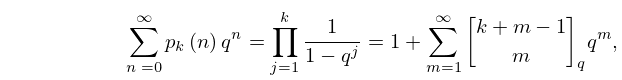
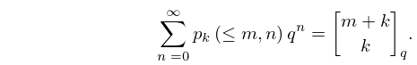
2: 26.9 Integer Partitions: Restricted Number and Part Size
…
►
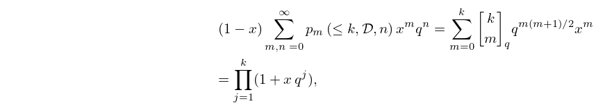
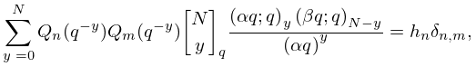
26.9.4
,
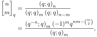
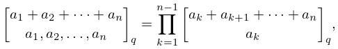
►is the Gaussian polynomial (or -binomial coefficient); see also §§17.2(i)–17.2(ii).
…
►
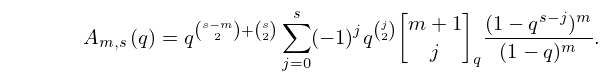
26.9.5
►
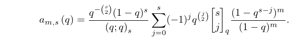
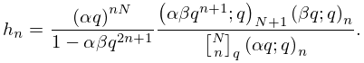
26.9.6
…
►
26.9.7
…
3: 17.2 Calculus
…
►
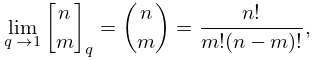
§17.2(ii) Binomial Coefficients
►
17.2.27
►
17.2.28
…
►
§17.2(iii) Binomial Theorem
… ►When , where is a nonnegative integer, (17.2.37) reduces to the -binomial series …4: 26.10 Integer Partitions: Other Restrictions
…
►
Table 26.10.1: Partitions restricted by difference conditions, or equivalently with parts from .
►
►
►
…
►
| … | ||||
26.10.3
,
…
5: Bibliography K
…
►
Algorithm 737: INTLIB: A portable Fortran 77 interval standard-function library.
ACM Trans. Math. Software 20 (4), pp. 447–459.
…
►
Methods of computing the Riemann zeta-function and some generalizations of it.
USSR Comput. Math. and Math. Phys. 20 (6), pp. 212–230.
…
►
Connection formulae for asymptotics of solutions of the degenerate third Painlevé equation. I.
Inverse Problems 20 (4), pp. 1165–1206.
…
►
The Askey scheme as a four-manifold with corners.
Ramanujan J. 20 (3), pp. 409–439.
…
►
HYP and HYPQ. Mathematica packages for the manipulation of binomial sums and hypergeometric series respectively -binomial sums and basic hypergeometric series.
Séminaire Lotharingien de Combinatoire 30, pp. 61–76.
…
6: 17.3 -Elementary and -Special Functions
7: 26.16 Multiset Permutations
…
►
26.16.1
…
8: 18.27 -Hahn Class
9: 6.20 Approximations
…
►
•
►
•
►
•
►
•
…
Cody and Thacher (1968) provides minimax rational approximations for , with accuracies up to 20S.
Cody and Thacher (1969) provides minimax rational approximations for , with accuracies up to 20S.
MacLeod (1996b) provides rational approximations for the sine and cosine integrals and for the auxiliary functions and , with accuracies up to 20S.
§6.20(ii) Expansions in Chebyshev Series
… ►Luke and Wimp (1963) covers for (20D), and and for (20D).
10: 25.20 Approximations
…
►
•
►
•
►
•
…
►
•
Cody et al. (1971) gives rational approximations for in the form of quotients of polynomials or quotients of Chebyshev series. The ranges covered are , , , . Precision is varied, with a maximum of 20S.
Piessens and Branders (1972) gives the coefficients of the Chebyshev-series expansions of and , , for (23D).
