q-binomial theorem

SearchAdvancedHelp

(0.004 seconds)

1—10 of 124 matching pages

1: 17.5 ${}_0{}^{}\varphi _0^{},{}_1{}^{}\varphi _0^{},{}_1{}^{}\varphi _1^{}$ Functions

… ►

$q$-Binomial Series

… ►

$q$-Binomial Theorem

…

2: 17.2 Calculus

… ►

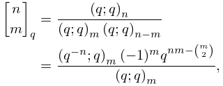
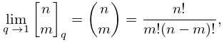
§17.2(ii) Binomial Coefficients

►

17.2.27 $${\left[\genfrac{}{}{0.0pt}{}{n}{m}\right]}_q=\frac{{(q;q)}_n}{{(q;q)}_m{(q;q)}_{n-m}}=\frac{{(q^{-n};q)}_m{(-1)}^m{q}^{nm-\left(\genfrac{}{}{0.0pt}{}{m}{2}\right)}}{{(q;q)}_m},$$

ⓘ

Defines:

${\left[\genfrac{}{}{0.0pt}{}{n}{m}\right]}_q$: $q$-binomial coefficient (or Gaussian polynomial)

Symbols:

$\left(\genfrac{}{}{0.0pt}{}{m}{n}\right)$: binomial coefficient, ${(a;q)}_n$: $q$-Pochhammer symbol (or $q$-shifted factorial), $q$: complex base, $m$: nonnegative integer and $n$: nonnegative integer

Permalink:

http://dlmf.nist.gov/17.2.E27

Encodings:

pMML, png, TeX

See also:

Annotations for §17.2(ii), §17.2 and Ch.17

►

17.2.28 $$\underset{q\to 1}{lim}{\left[\genfrac{}{}{0.0pt}{}{n}{m}\right]}_q=\left(\genfrac{}{}{0.0pt}{}{n}{m}\right)=\frac{n!}{m!(n-m)!},$$

ⓘ

Symbols:

$\left(\genfrac{}{}{0.0pt}{}{m}{n}\right)$: binomial coefficient, $!$: factorial (as in $n!$), ${\left[\genfrac{}{}{0.0pt}{}{n}{m}\right]}_q$: $q$-binomial coefficient (or Gaussian polynomial), $q$: complex base, $m$: nonnegative integer and $n$: nonnegative integer

Permalink:

http://dlmf.nist.gov/17.2.E28

Encodings:

pMML, png, TeX

See also:

Annotations for §17.2(ii), §17.2 and Ch.17

… ►

§17.2(iii) Binomial Theorem

… ►When $a=q^{m+1}$, where $m$ is a nonnegative integer, (17.2.37) reduces to the $q$-binomial series …

3: 26.9 Integer Partitions: Restricted Number and Part Size

… ►

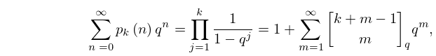
26.9.4 $${\left[\genfrac{}{}{0.0pt}{}{m}{n}\right]}_q=\prod _{j=1}^n\frac{1-q^{m-n+j}}{1-q^j},$$ $n\ge 0$,

ⓘ

Symbols:

${\left[\genfrac{}{}{0.0pt}{}{n}{m}\right]}_q$: $q$-binomial coefficient (or Gaussian polynomial), $j$: nonnegative integer, $m$: nonnegative integer, $n$: nonnegative integer and $q$: parameter

Permalink:

http://dlmf.nist.gov/26.9.E4

Encodings:

pMML, png, TeX

See also:

Annotations for §26.9(ii), §26.9 and Ch.26

►is the Gaussian polynomial (or $q$-binomial coefficient); see also §§17.2(i)–17.2(ii). … ►

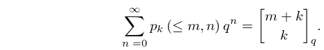
26.9.5 $$\sum _{n=0}^{\mathrm{\infty }}{p}_k\left(n\right)q^n=\prod _{j=1}^k\frac{1}{1-q^j}=1+\sum _{m=1}^{\mathrm{\infty }}{\left[\genfrac{}{}{0.0pt}{}{k+m-1}{m}\right]}_q{q}^m,$$

ⓘ

Symbols:

$p_k\left(n\right)$: total number of partitions of $n$ into at most $k$ parts, ${\left[\genfrac{}{}{0.0pt}{}{n}{m}\right]}_q$: $q$-binomial coefficient (or Gaussian polynomial), $j$: nonnegative integer, $k$: nonnegative integer, $m$: nonnegative integer, $n$: nonnegative integer and $q$: parameter

Permalink:

http://dlmf.nist.gov/26.9.E5

Encodings:

pMML, png, TeX

See also:

Annotations for §26.9(ii), §26.9 and Ch.26

►

26.9.6 $$\sum _{n=0}^{\mathrm{\infty }}{p}_k(\le m,n)q^n={\left[\genfrac{}{}{0.0pt}{}{m+k}{k}\right]}_q.$$

ⓘ

Symbols:

${\left[\genfrac{}{}{0.0pt}{}{n}{m}\right]}_q$: $q$-binomial coefficient (or Gaussian polynomial), $p_k(\le m,n)$: number of partitions of $n$ into at most $k$ parts, each less than or equal to $m$ , $k$: nonnegative integer, $m$: nonnegative integer, $n$: nonnegative integer and $q$: parameter

Permalink:

http://dlmf.nist.gov/26.9.E6

Encodings:

pMML, png, TeX

See also:

Annotations for §26.9(ii), §26.9 and Ch.26

… ►

26.9.7 $$\sum _{m,n=0}^{\mathrm{\infty }}{p}_k(\le m,n)x^k{q}^n=1+\sum _{k=1}^{\mathrm{\infty }}{\left[\genfrac{}{}{0.0pt}{}{m+k}{k}\right]}_q{x}^k=\prod _{j=0}^m\frac{1}{1-x{q}^j}.$$

ⓘ

Symbols:

${\left[\genfrac{}{}{0.0pt}{}{n}{m}\right]}_q$: $q$-binomial coefficient (or Gaussian polynomial), $p_k(\le m,n)$: number of partitions of $n$ into at most $k$ parts, each less than or equal to $m$ , $x$: real variable, $j$: nonnegative integer, $k$: nonnegative integer, $m$: nonnegative integer, $n$: nonnegative integer and $q$: parameter

Permalink:

http://dlmf.nist.gov/26.9.E7

Encodings:

pMML, png, TeX

See also:

Annotations for §26.9(ii), §26.9 and Ch.26

…

4: Bibliography K

… ►

An extension of Saalschütz’s summation theorem for the series ${}_{r+3}{}^{}F_{r+2}^{}$ . Integral Transforms Spec. Funct. 24 (11), pp. 916–921.

ⓘ

External Links:

ISSN 1065-2469, Document, FullText, MathReview (Christian Lavault), ZentralBlatt

Referenced by:

§16.4(ii), §16.4(ii).

Encodings:

BibTeX

… ►

A general addition theorem for spheroidal wave functions. SIAM J. Math. Anal. 4 (1), pp. 149–160.

ⓘ

External Links:

Document, MathReview (J. Meixner), ZentralBlatt

Referenced by:

§30.10.

Encodings:

BibTeX

… ►

A new proof of a Paley-Wiener type theorem for the Jacobi transform. Ark. Mat. 13, pp. 145–159.

ⓘ

External Links:

Document, MathReview (G. Gasper), ZentralBlatt

Referenced by:

§18.10(i).

Encodings:

BibTeX

… ►

HYP and HYPQ. Mathematica packages for the manipulation of binomial sums and hypergeometric series respectively $q$-binomial sums and basic hypergeometric series. Séminaire Lotharingien de Combinatoire 30, pp. 61–76.

ⓘ

Notes:

Also published in J. Symbolic Comput. (1995), v. 20, no. 5–6, pp. 737–744.

External Links:

Code, Document, MathReview (G. Gasper), ZentralBlatt

Referenced by:

1st item.

Encodings:

BibTeX

…

5: 17.3 $q$-Elementary and $q$-Special Functions

… ►

17.3.8 $$A_{m,s}\left(q\right)=q^{\left(\genfrac{}{}{0.0pt}{}{s-m}{2}\right)+\left(\genfrac{}{}{0.0pt}{}{s}{2}\right)}\sum _{j=0}^s{(-1)}^j{q}^{\left(\genfrac{}{}{0.0pt}{}{j}{2}\right)}{\left[\genfrac{}{}{0.0pt}{}{m+1}{j}\right]}_q\frac{{(1-q^{s-j})}^m}{{(1-q)}^m}.$$

ⓘ

Defines:

$A_{m,s}\left(q\right)$: $q$-Euler number

Symbols:

$\left(\genfrac{}{}{0.0pt}{}{m}{n}\right)$: binomial coefficient, ${\left[\genfrac{}{}{0.0pt}{}{n}{m}\right]}_q$: $q$-binomial coefficient (or Gaussian polynomial), $q$: complex base, $j$: nonnegative integer, $m$: nonnegative integer and $s$: nonnegative integer

Permalink:

http://dlmf.nist.gov/17.3.E8

Encodings:

pMML, png, TeX

See also:

Annotations for §17.3(iii), §17.3(iii), §17.3 and Ch.17

… ►

17.3.9 $$a_{m,s}\left(q\right)=\frac{q^{-\left(\genfrac{}{}{0.0pt}{}{s}{2}\right)}{(1-q)}^s}{{(q;q)}_s}\sum _{j=0}^s{(-1)}^j{q}^{\left(\genfrac{}{}{0.0pt}{}{j}{2}\right)}{\left[\genfrac{}{}{0.0pt}{}{s}{j}\right]}_q\frac{{(1-q^{s-j})}^m}{{(1-q)}^m}.$$

ⓘ

Defines:

$a_{m,s}\left(q\right)$: $q$-Stirling number

Symbols:

$\left(\genfrac{}{}{0.0pt}{}{m}{n}\right)$: binomial coefficient, ${(a;q)}_n$: $q$-Pochhammer symbol (or $q$-shifted factorial), ${\left[\genfrac{}{}{0.0pt}{}{n}{m}\right]}_q$: $q$-binomial coefficient (or Gaussian polynomial), $q$: complex base, $j$: nonnegative integer, $m$: nonnegative integer and $s$: nonnegative integer

Permalink:

http://dlmf.nist.gov/17.3.E9

Encodings:

pMML, png, TeX

See also:

Annotations for §17.3(iii), §17.3(iii), §17.3 and Ch.17

…

6: 26.16 Multiset Permutations

… ►

26.16.1 $${\left[\genfrac{}{}{0.0pt}{}{a_1+a_2+\mathrm{\cdots }+a_n}{a_1,a_2,\mathrm{\dots },a_n}\right]}_q=\prod _{k=1}^{n-1}{\left[\genfrac{}{}{0.0pt}{}{a_k+a_{k+1}+\mathrm{\cdots }+a_n}{a_k}\right]}_q,$$

ⓘ

Symbols:

${\left[\genfrac{}{}{0.0pt}{}{n}{m}\right]}_q$: $q$-binomial coefficient (or Gaussian polynomial), ${\left[\genfrac{}{}{0.0pt}{}{a_1+a_2+\mathrm{\cdots }+a_n}{a_1,a_2,\mathrm{\dots },a_n}\right]}_q$: $q$-multinomial coefficient, $k$: nonnegative integer, $n$: nonnegative integer, $a_j$: numbers and $q$: parameter

Permalink:

http://dlmf.nist.gov/26.16.E1

Encodings:

pMML, png, TeX

See also:

Annotations for §26.16 and Ch.26

…

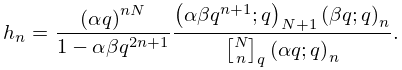
7: 18.27 $q$-Hahn Class

… ►

18.27.4 $$\sum _{y=0}^N{Q}_n(q^{-y})Q_m(q^{-y}){\left[\genfrac{}{}{0.0pt}{}{N}{y}\right]}_q\frac{{(\alpha q;q)}_y{(\beta q;q)}_{N-y}}{{\left(\alpha q\right)}^y}=h_n{\delta }_{n,m},$$ $n,m=0,1,\mathrm{\dots },N$,

ⓘ

Symbols:

${\delta }_{j,k}$: Kronecker delta, ${(a;q)}_n$: $q$-Pochhammer symbol (or $q$-shifted factorial), ${\left[\genfrac{}{}{0.0pt}{}{n}{m}\right]}_q$: $q$-binomial coefficient (or Gaussian polynomial), $y$: real variable, $N$: positive integer, $q$: real variable, $m$: nonnegative integer, $n$: nonnegative integer and $h_n$

Notes:

This is Ismail (2009, (18.5.2)) but the presentation has been simplified.

Referenced by:

§18.27(ii), Erratum (V1.2.0) for Equation (18.27.4)

Permalink:

http://dlmf.nist.gov/18.27.E4

Encodings:

pMML, png, TeX

Correction (effective with 1.1.2):

$q$-Pochhammer symbols now link to their definition.

See also:

Annotations for §18.27(ii), §18.27 and Ch.18

… ►

18.27.4_1 $$h_n=\frac{{\left(\alpha q\right)}^{nN}}{1-\alpha \beta q^{2n+1}}\frac{{(\alpha \beta q^{n+1};q)}_{N+1}{(\beta q;q)}_n}{{\left[\genfrac{}{}{0.0pt}{}{N}{n}\right]}_q{(\alpha q;q)}_n}.$$

ⓘ

Symbols:

${(a;q)}_n$: $q$-Pochhammer symbol (or $q$-shifted factorial), ${\left[\genfrac{}{}{0.0pt}{}{n}{m}\right]}_q$: $q$-binomial coefficient (or Gaussian polynomial), $N$: positive integer, $q$: real variable, $n$: nonnegative integer and $h_n$

Referenced by:

§18.27(ii), Erratum (V1.2.0) Section 18.27

Permalink:

http://dlmf.nist.gov/18.27.E4_1

Encodings:

pMML, png, TeX

Addition (effective with 1.2.0):

This equation was added.

See also:

Annotations for §18.27(ii), §18.27 and Ch.18

…

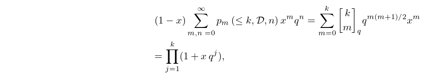
8: 26.10 Integer Partitions: Other Restrictions

… ►

26.10.3 $$(1-x)\sum _{m,n=0}^{\mathrm{\infty }}{p}_m(\le k,𝒟,n)x^m{q}^n=\sum _{m=0}^k{\left[\genfrac{}{}{0.0pt}{}{k}{m}\right]}_q{q}^{m(m+1)/2}{x}^m=\prod _{j=1}^k(1+x{q}^j),$$ ,

ⓘ

Symbols:

${\left[\genfrac{}{}{0.0pt}{}{n}{m}\right]}_q$: $q$-binomial coefficient (or Gaussian polynomial), $p_k(\le m,n)$: number of partitions of $n$ into at most $k$ parts, each less than or equal to $m$ , $x$: real variable, $j$: nonnegative integer, $k$: nonnegative integer, $m$: nonnegative integer, $n$: nonnegative integer and $q$: parameter

Referenced by:

§26.10(ii)

Permalink:

http://dlmf.nist.gov/26.10.E3

Encodings:

pMML, png, TeX

See also:

Annotations for §26.10(ii), §26.10 and Ch.26

…

9: 28.27 Addition Theorems

§28.27 Addition Theorems

►Addition theorems provide important connections between Mathieu functions with different parameters and in different coordinate systems. They are analogous to the addition theorems for Bessel functions (§10.23(ii)) and modified Bessel functions (§10.44(ii)). …

10: 27.15 Chinese Remainder Theorem

§27.15 Chinese Remainder Theorem

►The Chinese remainder theorem states that a system of congruences $x\equiv a_1(mod{m}_1),\mathrm{\dots },x\equiv a_k(mod{m}_k)$, always has a solution if the moduli are relatively prime in pairs; the solution is unique (mod $m$), where $m$ is the product of the moduli. ►This theorem is employed to increase efficiency in calculating with large numbers by making use of smaller numbers in most of the calculation. …By the Chinese remainder theorem each integer in the data can be uniquely represented by its residues (mod $m_1$), (mod $m_2$), (mod $m_3$), and (mod $m_4$), respectively. …These numbers, in turn, are combined by the Chinese remainder theorem to obtain the final result $(modm)$, which is correct to 20 digits. …