q-Racah polynomials

SearchAdvancedHelp

(0.003 seconds)

1—10 of 255 matching pages

1: 31.5 Solutions Analytic at Three Singularities: Heun Polynomials

§31.5 Solutions Analytic at Three Singularities: Heun Polynomials

… ►

31.5.2 $${\mathrm{𝐻𝑝}}_{n,m}(a,q_{n,m};-n,\beta ,\gamma ,\delta ;z)=H\mathrm{\ell }(a,q_{n,m};-n,\beta ,\gamma ,\delta ;z)$$

ⓘ

Defines:

${\mathrm{𝐻𝑝}}_{n,m}(a,q_{n,m};-n,\beta ,\gamma ,\delta ;z)$: Heun polynomials

Symbols:

$H\mathrm{\ell }(a,q;\alpha ,\beta ,\gamma ,\delta ;z)$: Heun functions, $z$: complex variable, $\gamma$: real or complex parameter, $\delta$: real or complex parameter, $m$: nonnegative integer, $n$: nonnegative integer, $a$: complex parameter, $q$: real or complex parameter and $\beta$: real or complex parameter

Permalink:

http://dlmf.nist.gov/31.5.E2

Encodings:

pMML, png, TeX

See also:

Annotations for §31.5 and Ch.31

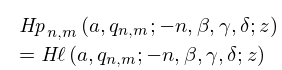
►is a polynomial of degree $n$, and hence a solution of (31.2.1) that is analytic at all three finite singularities $0,1,a$. These solutions are the Heun polynomials. …

2: 35.4 Partitions and Zonal Polynomials

§35.4 Partitions and Zonal Polynomials

… ►

Normalization

… ►

Orthogonal Invariance

… ►

Summation

… ►

Mean-Value

…

3: 24.1 Special Notation

… ►

Bernoulli Numbers and Polynomials

►The origin of the notation $B_n$, $B_n\left(x\right)$, is not clear. … ►

Euler Numbers and Polynomials

… ►The notations $E_n$, $E_n\left(x\right)$, as defined in §24.2(ii), were used in Lucas (1891) and Nörlund (1924). …

4: 18.3 Definitions

§18.3 Definitions

… ►For expressions of ultraspherical, Chebyshev, and Legendre polynomials in terms of Jacobi polynomials, see §18.7(i). …For explicit power series coefficients up to $n=12$ for these polynomials and for coefficients up to $n=6$ for Jacobi and ultraspherical polynomials see Abramowitz and Stegun (1964, pp. 793–801). … ►

Bessel polynomials

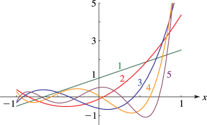
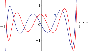
►Bessel polynomials are often included among the classical OP’s. …

5: 24.18 Physical Applications

§24.18 Physical Applications

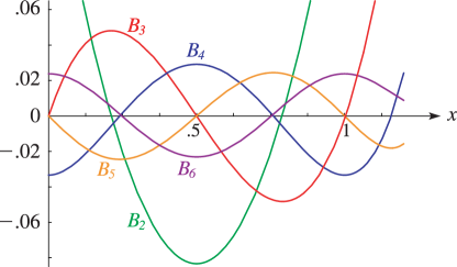
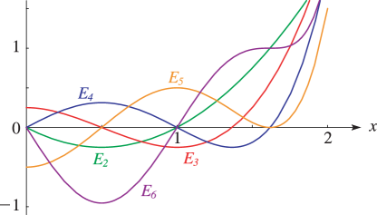
►Bernoulli polynomials appear in statistical physics (Ordóñez and Driebe (1996)), in discussions of Casimir forces (Li et al. (1991)), and in a study of quark-gluon plasma (Meisinger et al. (2002)). ►Euler polynomials also appear in statistical physics as well as in semi-classical approximations to quantum probability distributions (Ballentine and McRae (1998)).

6: 24.3 Graphs

… ►

►►

Figure 24.3.1: Bernoulli polynomials $B_n\left(x\right)$, $n=2,3,\mathrm{\dots },6$. Magnify

►

►►

Figure 24.3.2: Euler polynomials $E_n\left(x\right)$, $n=2,3,\mathrm{\dots },6$. Magnify

7: 18.4 Graphics

… ►

►►

Figure 18.4.1: Jacobi polynomials $P_n^{(1.5,-0.5)}\left(x\right)$, $n=1,2,3,4,5$. Magnify

►

►►

Figure 18.4.2: Jacobi polynomials $P_n^{(1.25,0.75)}\left(x\right)$, $n=7,8$. … Magnify

… ►

►►

Figure 18.4.4: Legendre polynomials $P_n\left(x\right)$, $n=1,2,3,4,5$. Magnify

►

►►

Figure 18.4.5: Laguerre polynomials $L_n\left(x\right)$, $n=1,2,3,4,5$. Magnify

… ►

►►

Figure 18.4.7: Monic Hermite polynomials $h_n(x)=2^{-n}{H}_n\left(x\right)$, $n=1,2,3,4,5$. Magnify

…

8: 18.7 Interrelations and Limit Relations

§18.7 Interrelations and Limit Relations

… ►

Chebyshev, Ultraspherical, and Jacobi

… ►

Legendre, Ultraspherical, and Jacobi

… ►

§18.7(ii) Quadratic Transformations

… ►

§18.7(iii) Limit Relations

…

9: 18.41 Tables

… ►

§18.41(i) Polynomials

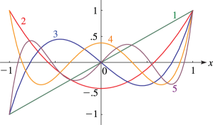
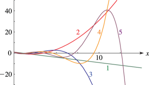
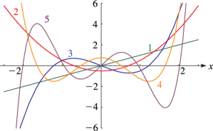
►For $P_n\left(x\right)$ ($={𝖯}_n\left(x\right)$) see §14.33. ►Abramowitz and Stegun (1964, Tables 22.4, 22.6, 22.11, and 22.13) tabulates $T_n\left(x\right)$, $U_n\left(x\right)$, $L_n\left(x\right)$, and $H_n\left(x\right)$ for $n=0(1)12$. The ranges of $x$ are $0.2(.2)1$ for $T_n\left(x\right)$ and $U_n\left(x\right)$, and $0.5,1,3,5,10$ for $L_n\left(x\right)$ and $H_n\left(x\right)$. … ►For $P_n\left(x\right)$, $L_n\left(x\right)$, and $H_n\left(x\right)$ see §3.5(v). …

10: 18.6 Symmetry, Special Values, and Limits to Monomials

… ►For Jacobi, ultraspherical, Chebyshev, Legendre, and Hermite polynomials, see Table 18.6.1. ►

Laguerre

… ►

Table 18.6.1: Classical OP’s: symmetry and special values.

► ►►

$p_n(x)$	$p_n(-x)$	$p_n(1)$	$p_{2n}(0)$	$p_{2n+1}^{\prime }(0)$
…

►

►

§18.6(ii) Limits to Monomials

… ►

18.6.4 $$\underset{\lambda \to \mathrm{\infty }}{lim}\frac{C_n^{(\lambda )}\left(x\right)}{C_n^{(\lambda )}\left(1\right)}=x^n,$$

ⓘ

Symbols:

$C_n^{(\lambda )}\left(x\right)$: ultraspherical (or Gegenbauer) polynomial, $n$: nonnegative integer and $x$: real variable

Referenced by:

§18.18(iv), §18.6(ii)

Permalink:

http://dlmf.nist.gov/18.6.E4

Encodings:

pMML, png, TeX

See also:

Annotations for §18.6(ii), §18.6 and Ch.18

…