punctured neighborhood

SearchAdvancedHelp

(0.001 seconds)

11—20 of 29 matching pages

11: 31.7 Relations to Other Functions

… ►Similar specializations of formulas in §31.3(ii) yield solutions in the neighborhoods of the singularities $\zeta =K$, $K+\mathrm{i}{K}^{\prime }$, and $\mathrm{i}{K}^{\prime }$, where $K$ and $K^{\prime }$ are related to $k$ as in §19.2(ii).

12: 15.10 Hypergeometric Differential Equation

… ►They are also numerically satisfactory (§2.7(iv)) in the neighborhood of the corresponding singularity. … ►(a) If $c$ equals $n=1,2,3,\mathrm{\dots }$, and $a=1,2,\mathrm{\dots },n-1$, then fundamental solutions in the neighborhood of $z=0$ are given by (15.10.2) with the interpretation (15.2.5) for $f_2(z)$. ►(b) If $c$ equals $n=1,2,3,\mathrm{\dots }$, and $a\ne 1,2,\mathrm{\dots },n-1$, then fundamental solutions in the neighborhood of $z=0$ are given by $F(a,b;n;z)$ and … ►(c) If the parameter $c$ in the differential equation equals $2-n=0,-1,-2,\mathrm{\dots }$, then fundamental solutions in the neighborhood of $z=0$ are given by $z^{n-1}$ times those in (a) and (b), with $a$ and $b$ replaced throughout by $a+n-1$ and $b+n-1$, respectively. ►(d) If $a+b+1-c$ equals $n=1,2,3,\mathrm{\dots }$, or $2-n=0,-1,-2,\mathrm{\dots }$, then fundamental solutions in the neighborhood of $z=1$ are given by those in (a), (b), and (c) with $z$ replaced by $1-z$. …

13: 1.4 Calculus of One Variable

… ►A necessary condition that a differentiable function $f(x)$ has a local maximum (minimum) at $x=c$, that is, $f(x)\le f(c)$, ($f(x)\ge f(c)$) in a neighborhood $c-\delta \le x\le c+\delta$ ($\delta >0$) of $c$, is $f^{\prime }(c)=0$. … ►We do assume that $g^{\prime }(x)\ne 0$ for all $x$ in some neighborhood of $a$ with $x\ne a$. …

14: 1.5 Calculus of Two or More Variables

… ►

Implicit Function Theorem

►If $F(x,y)$ is continuously differentiable, $F(a,b)=0$, and $\partial F/\partial y\ne 0$ at $(a,b)$, then in a neighborhood of $(a,b)$, that is, an open disk centered at $a,b$, the equation $F(x,y)=0$ defines a continuously differentiable function $y=g(x)$ such that $F(x,g(x))=0$, $b=g(a)$, and $g^{\prime }(x)=-F_x/F_y$. …

15: Bibliography

… ►

Normal forms of functions in the neighborhood of degenerate critical points. Uspehi Mat. Nauk 29 (2(176)), pp. 11–49 (Russian).

ⓘ

Notes:

Collection of articles dedicated to the memory of Ivan Georgievič Petrovskiĭ (1901–1973), I. In Russian. English translation: Russian Math. Surveys, 29(1974), no. 2, pp. 10–50.

External Links:

Document, MathReview (G. R. Belickii), ZentralBlatt

Referenced by:

§36.2(i).

Encodings:

BibTeX

…

16: 3.7 Ordinary Differential Equations

… ►For classification of singularities of (3.7.1) and expansions of solutions in the neighborhoods of singularities, see §2.7. …

17: 33.14 Definitions and Basic Properties

… ►This includes $ϵ=0$, hence $f(ϵ,\mathrm{\ell };r)$ can be expanded in a convergent power series in $ϵ$ in a neighborhood of $ϵ=0$ (§33.20(ii)). …

18: 1.14 Integral Transforms

… ►Suppose that $f(t)$ is absolutely integrable on $(-\mathrm{\infty },\mathrm{\infty })$ and of bounded variation in a neighborhood of $t=u$ (§1.4(v)). … ►If $f(t)$ is absolutely integrable on $[0,\mathrm{\infty })$ and of bounded variation (§1.4(v)) in a neighborhood of $t=u$, then … ►Suppose the integral (1.14.32) is absolutely convergent on the line $\mathrm{\Re }s=\sigma$ and $f(x)$ is of bounded variation in a neighborhood of $x=u$. …

19: 1.13 Differential Equations

… ►For classification of singularities of (1.13.1) and expansions of solutions in the neighborhoods of singularities, see §2.7. …

20: 2.4 Contour Integrals

… ►

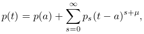
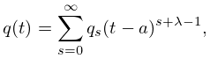
In a neighborhood of $a$

2.4.11

$$p(t)=p(a)+\sum _{s=0}^{\mathrm{\infty }}{p}_s{(t-a)}^{s+\mu },$$

$$q(t)=\sum _{s=0}^{\mathrm{\infty }}{q}_s{(t-a)}^{s+\lambda -1},$$

ⓘ

Symbols:

$\lambda$: constant, $a$: left endpoint, $p(t)$: analytic function, $q(t)$: analytic function, $p_s$: coefficients, $q_s$: coefficients and $\mu$: positive constant

Referenced by:

§2.4(iv)

Permalink:

http://dlmf.nist.gov/2.4.E11

Encodings:

pMML, pMML, png, png, TeX, TeX

See also:

Annotations for §2.4(iii), §2.4 and Ch.2

with $\mathrm{\Re }\lambda >0$, $\mu >0$, $p_0\ne 0$, and the branches of ${(t-a)}^{\lambda }$ and ${(t-a)}^{\mu }$ continuous and constructed with $\mathrm{ph}\left(t-a\right)\to \omega$ as $t\to a$ along $𝒫$.

…