psi%20function

SearchAdvancedHelp

(0.003 seconds)

1—10 of 14 matching pages

1: 9.18 Tables

… ►

Miller (1946) tabulates $\mathrm{Ai}\left(x\right)$, ${\mathrm{Ai}}^{\prime }\left(x\right)$ for $x=-20(.01)2;$ ${\log }_{10}\mathrm{Ai}\left(x\right)$, ${\mathrm{Ai}}^{\prime }\left(x\right)/\mathrm{Ai}\left(x\right)$ for $x=0(.1)25(1)75$; $\mathrm{Bi}\left(x\right)$, ${\mathrm{Bi}}^{\prime }\left(x\right)$ for $x=-10(.1)2.5$; ${\log }_{10}\mathrm{Bi}\left(x\right)$, ${\mathrm{Bi}}^{\prime }\left(x\right)/\mathrm{Bi}\left(x\right)$ for $x=0(.1)10$; $M\left(x\right)$, $N\left(x\right)$, $\theta \left(x\right)$, $\varphi \left(x\right)$ (respectively $F(x)$, $G(x)$, $\chi (x)$, $\psi (x)$) for $x=-80(1)-30(.1)0$. Precision is generally 8D; slightly less for some of the auxiliary functions. Extracts from these tables are included in Abramowitz and Stegun (1964, Chapter 10), together with some auxiliary functions for large arguments.

…

2: 36.2 Catastrophes and Canonical Integrals

… ►

36.2.28 $${\mathrm{\Psi }}^{(\mathrm{E})}\left(0,0,z\right)=\overline{{\mathrm{\Psi }}^{(\mathrm{E})}\left(0,0,-z\right)}=2\pi \sqrt{\frac{\pi z}{27}}\exp \left(\frac{2}{27}\mathrm{i}{z}^3\right)\left(J_{-1/6}\left(\frac{2}{27}{z}^3\right)+\mathrm{i}{J}_{1/6}\left(\frac{2}{27}{z}^3\right)\right),$$ $z\ge 0$,

ⓘ

Symbols:

$J_{\nu }\left(z\right)$: Bessel function of the first kind, $\pi$: the ratio of the circumference of a circle to its diameter, $\overline{z}$: complex conjugate, ${\mathrm{\Psi }}^{(\mathrm{E})}\left(𝐱\right)$: elliptic umbilic canonical integral function, $\exp z$: exponential function, $\mathrm{i}$: imaginary unit and $z$: real parameter

Referenced by:

Erratum (V1.0.5) for Chapters 8, 20, 36

Permalink:

http://dlmf.nist.gov/36.2.E28

Encodings:

pMML, png, TeX

Addition (effective with 1.0.5):

This equation has been added. For the proof see Berry and Howls (2010).

See also:

Annotations for §36.2(iv), §36.2 and Ch.36

►

36.2.29 $${\mathrm{\Psi }}^{(\mathrm{H})}\left(0,0,z\right)=\overline{{\mathrm{\Psi }}^{(\mathrm{H})}\left(0,0,-z\right)}=\frac{2^{1/3}}{\sqrt{3}}\exp \left(\frac{1}{27}\mathrm{i}{z}^3\right){\mathrm{\Psi }}^{(\mathrm{E})}\left(0,0,-\frac{z}{2^{2/3}}\right),$$ .

ⓘ

Symbols:

$\overline{z}$: complex conjugate, ${\mathrm{\Psi }}^{(\mathrm{E})}\left(𝐱\right)$: elliptic umbilic canonical integral function, $\exp z$: exponential function, ${\mathrm{\Psi }}^{(\mathrm{H})}\left(𝐱\right)$: hyperbolic umbilic canonical integral function, $\mathrm{i}$: imaginary unit and $z$: real parameter

Referenced by:

Erratum (V1.0.5) for Chapters 8, 20, 36

Permalink:

http://dlmf.nist.gov/36.2.E29

Encodings:

pMML, png, TeX

Addition (effective with 1.0.5):

This equation has been added. For the proof see Berry and Howls (2010).

See also:

Annotations for §36.2(iv), §36.2 and Ch.36

3: 5.22 Tables

… ►

§5.22(ii) Real Variables

►Abramowitz and Stegun (1964, Chapter 6) tabulates $\mathrm{\Gamma }\left(x\right)$, $\ln \mathrm{\Gamma }\left(x\right)$, $\psi \left(x\right)$, and ${\psi }^{\prime }\left(x\right)$ for $x=1(.005)2$ to 10D; ${\psi }^{\prime \prime }\left(x\right)$ and ${\psi }^{(3)}\left(x\right)$ for $x=1(.01)2$ to 10D; $\mathrm{\Gamma }\left(n\right)$, $1/\mathrm{\Gamma }\left(n\right)$, $\mathrm{\Gamma }\left(n+\frac{1}{2}\right)$, $\psi \left(n\right)$, ${\log }_{10}\mathrm{\Gamma }\left(n\right)$, ${\log }_{10}\mathrm{\Gamma }\left(n+\frac{1}{3}\right)$, ${\log }_{10}\mathrm{\Gamma }\left(n+\frac{1}{2}\right)$, and ${\log }_{10}\mathrm{\Gamma }\left(n+\frac{2}{3}\right)$ for $n=1(1)101$ to 8–11S; $\mathrm{\Gamma }\left(n+1\right)$ for $n=100(100)1000$ to 20S. Zhang and Jin (1996, pp. 67–69 and 72) tabulates $\mathrm{\Gamma }\left(x\right)$, $1/\mathrm{\Gamma }\left(x\right)$, $\mathrm{\Gamma }\left(-x\right)$, $\ln \mathrm{\Gamma }\left(x\right)$, $\psi \left(x\right)$, $\psi \left(-x\right)$, ${\psi }^{\prime }\left(x\right)$, and ${\psi }^{\prime }\left(-x\right)$ for $x=0(.1)5$ to 8D or 8S; $\mathrm{\Gamma }\left(n+1\right)$ for $n=0(1)100(10)250(50)500(100)3000$ to 51S. ►

§5.22(iii) Complex Variables

… ►This reference also includes $\psi \left(x+\mathrm{i}y\right)$ for the same arguments to 5D. …

4: Bibliography D

… ►

Recherches analytiques sur la théorie des nombres premiers. Première partie. La fonction $\zeta (s)$ de Riemann et les nombres premiers en général, suivi d’un Appendice sur des réflexions applicables à une formule donnée par Riemann. Ann. Soc. Sci. Bruxelles 20, pp. 183–256 (French).

ⓘ

Notes:

Reprinted in Collected works/Oeuvres scientifiques, Vol. I, pp. 223–296 Académie Royale de Belgique, Brussels, 2000.

External Links:

MathReview, ZentralBlatt

Referenced by:

§25.10(i), §27.11, §27.2(i).

Encodings:

BibTeX

►

Recherches analytiques sur la théorie des nombres premiers. Deuxième partie. Les fonctions de Dirichlet et les nombres premiers de la forme linéaire $Mx+N$ . Ann. Soc. Sci. Bruxelles 20, pp. 281–397 (French).

ⓘ

Notes:

Reprinted in Collected works/Oeuvres scientifiques, Vol. I, pp. 309–425, Académie Royale de Belgique, Brussels, 2000.

External Links:

MathReview, ZentralBlatt

Referenced by:

§25.10(i), §27.11, §27.2(i).

Encodings:

BibTeX

… ►

Complex zeros of cylinder functions. Math. Comp. 20 (94), pp. 215–222.

ⓘ

Notes:

For a numerical error in one of the zeros see Amos (1985).

External Links:

ISSN 0025-5718, FullText, MathReview, ZentralBlatt

Referenced by:

2nd item.

Encodings:

BibTeX

… ►

Uniform asymptotic expansions for Whittaker’s confluent hypergeometric functions. SIAM J. Math. Anal. 20 (3), pp. 744–760.

ⓘ

Notes:

(This reference has several typographical errors.)

External Links:

ISSN 0036-1410, Document, MathReview (F. W. J. Olver), ZentralBlatt

Referenced by:

§13.21(ii), §13.21(iii), §13.21(iv).

Encodings:

BibTeX

►

Bessel functions of purely imaginary order, with an application to second-order linear differential equations having a large parameter. SIAM J. Math. Anal. 21 (4), pp. 995–1018.

ⓘ

Notes:

Errata: In eq. (2.8) replace ${(x^2/4)}^2$ by ${(x^2/4)}^s$. In eq. (4.2) $\varphi (\zeta )$ should be replaced by $\psi (\zeta )$. In the second line of eq. (4.7) insert an external factor $e^{-2\pi ij/3}$ and change the upper limit of the sum to $n-1$. In eq. (4.15) the factor $\zeta$ is missing from the arguments of the functions Bi_ν and Bi’_ν.

External Links:

ISSN 0036-1410, Document, MathReview (A. de Castro Brzezicki), ZentralBlatt

Referenced by:

§10.24, §10.45, §2.8(iv).

Encodings:

BibTeX

…

5: 10.73 Physical Applications

… ►Bessel functions of the first kind, $J_n\left(x\right)$, arise naturally in applications having cylindrical symmetry in which the physics is described either by Laplace’s equation ${\nabla }^{2}V=0$, or by the Helmholtz equation $({\nabla }^2+k^2)\psi =0$. … ►The Helmholtz equation, $({\nabla }^2+k^2)\psi =0$, follows from the wave equation …See Krivoshlykov (1994, Chapter 2, §2.2.10; Chapter 5, §5.2.2), Kapany and Burke (1972, Chapters 4–6; Chapter 7, §A.1), and Slater (1942, Chapter 4, §§20, 25). … ►

§10.73(iii) Kelvin Functions

… ►

§10.73(iv) Bickley Functions

…

6: 19.36 Methods of Computation

… ►When the differences are moderately small, the iteration is stopped, the elementary symmetric functions of certain differences are calculated, and a polynomial consisting of a fixed number of terms of the sum in (19.19.7) is evaluated. …where the elementary symmetric functions $E_s$ are defined by (19.19.4). … ►

§19.36(iii) Via Theta Functions

… ►For computation of Legendre’s integral of the third kind, see Abramowitz and Stegun (1964, §§17.7 and 17.8, Examples 15, 17, 19, and 20). … ►When the values of complete integrals are known, addition theorems with $\psi =\pi /2$ (§19.11(ii)) ease the computation of functions such as $F(\varphi ,k)$ when $\frac{1}{2}\pi -\varphi$ is small and positive. …

7: Errata

… ►

A sentence and unnumbered equation

$$R_C(\gamma -\delta ,\gamma )=\frac{-1}{\sqrt{\delta }}\arctan \left(\frac{\sqrt{\delta }\sin \theta \sin \varphi \sin \psi }{{\alpha }^2-1-{\alpha }^2\cos \theta \cos \varphi \cos \psi }\right),$$

were added which indicate that care must be taken with the multivalued functions in (19.11.5). See (Cayley, 1961, pp. 103-106).

Suggested by Albert Groenenboom.

… ►

Scales were corrected in all figures. The interval $-8.4\le \frac{x-y}{\sqrt{2}}\le 8.4$ was replaced by $-12.0\le \frac{x-y}{\sqrt{2}}\le 12.0$ and $-12.7\le \frac{x+y}{\sqrt{2}}\le 4.2$ replaced by $-18.0\le \frac{x+y}{\sqrt{2}}\le 6.0$. All plots and interactive visualizations were regenerated to improve image quality.

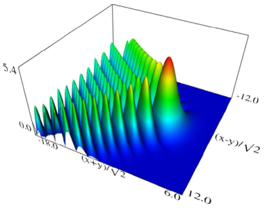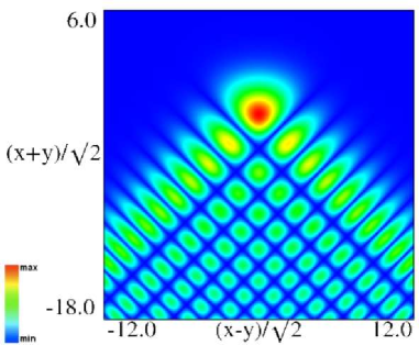
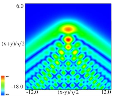
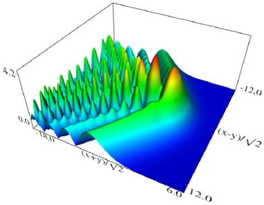
(a) Density plot.	(b) 3D plot.

Figure 36.3.9: Modulus of hyperbolic umbilic canonical integral function $|{\mathrm{\Psi }}^{(\mathrm{H})}\left(x,y,0\right)|$.

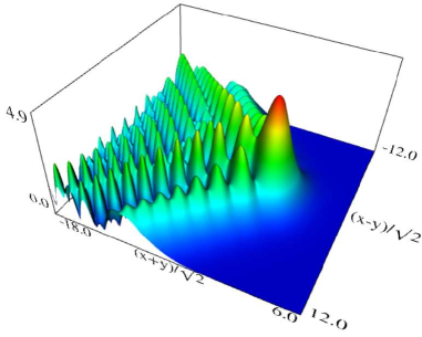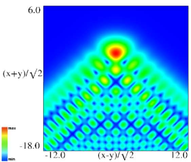
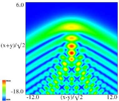
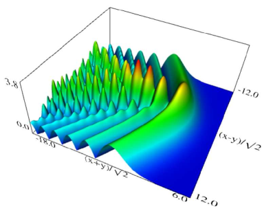
(a) Density plot.	(b) 3D plot.

Figure 36.3.10: Modulus of hyperbolic umbilic canonical integral function $|{\mathrm{\Psi }}^{(\mathrm{H})}\left(x,y,1\right)|$.

(a) Density plot.	(b) 3D plot.

Figure 36.3.11: Modulus of hyperbolic umbilic canonical integral function $|{\mathrm{\Psi }}^{(\mathrm{H})}\left(x,y,2\right)|$.

(a) Density plot.	(b) 3D plot.

Figure 36.3.12: Modulus of hyperbolic umbilic canonical integral function $|{\mathrm{\Psi }}^{(\mathrm{H})}\left(x,y,3\right)|$.

Reported 2016-09-12 by Dan Piponi.

… ►

31.8.5 $${\mathrm{\Psi }}_{1,-1}=\left(z^2+(\lambda +3a+3)z+a\right)/z^3$$

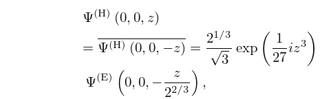
Originally the first term on the right side of the equation for ${\mathrm{\Psi }}_{1,-1}$ was $z^3$. The correct factor is $z^2$.

Reported 2013-07-25 by Christopher Künstler.

… ►

Several new equations have been added. See (8.17.24), (20.7.34), §20.11(v), (26.12.27), (36.2.28), and (36.2.29).

… ►

Bibliographic citations were added in §§1.13(v), 10.14, 10.21(ii), 18.15(v), 18.32, 30.16(iii), 32.13(ii), and as general references in Chapters 19, 20, 22, and 23.

…

8: Bibliography

… ►

Exact linearization of a Painlevé transcendent. Phys. Rev. Lett. 38 (20), pp. 1103–1106.

ⓘ

External Links:

Document, MathReview (Mark Adler)

Referenced by:

§32.11(ii), §32.13(i), §32.13(ii), §32.13(iii), §32.5.

Encodings:

BibTeX

… ►

On the degrees of irreducible factors of higher order Bernoulli polynomials. Acta Arith. 62 (4), pp. 329–342.

ⓘ

External Links:

ISSN 0065-1036, Pdf, MathReview (L. Skula), ZentralBlatt

Referenced by:

§24.12(iii).

Encodings:

BibTeX

… ►

Numerical computation of Tricomi’s psi function by the trapezoidal rule. Computing 39 (3), pp. 271–279.

ⓘ

External Links:

ISSN 0010-485X, Document, MathReview, ZentralBlatt

Referenced by:

§13.29(iii).

Encodings:

BibTeX

… ►

Algorithm 610. A portable FORTRAN subroutine for derivatives of the psi function. ACM Trans. Math. Software 9 (4), pp. 494–502.

ⓘ

Notes:

Single and double precision, maximum accuracy 18S.

External Links:

ISSN 0098-3500, Document, GAMS (module 610; package TOMS), MathReview Entry, ZentralBlatt

Referenced by:

1st item.

Encodings:

BibTeX

… ►

Repeated integrals and derivatives of $K$ Bessel functions. SIAM J. Math. Anal. 20 (1), pp. 169–175.

ⓘ

External Links:

ISSN 0036-1410, Document, MathReview (A. Haimovici), ZentralBlatt

Referenced by:

§10.43(iii).

Encodings:

BibTeX

…

9: 5.11 Asymptotic Expansions

§5.11 Asymptotic Expansions

… ►and … ►Wrench (1968) gives exact values of $g_k$ up to $g_{20}$. … ►

§5.11(iii) Ratios

… ►

10: Bibliography W

… ►

Evaluating elliptic functions and their inverses. Comput. Math. Appl. 39 (3-4), pp. 131–136.

ⓘ

External Links:

ISSN 0898-1221, Document, MathReview, ZentralBlatt

Referenced by:

§22.20(ii), §22.20(v).

Encodings:

BibTeX

… ►

Infinitely differentiable generalized logarithmic and exponential functions. Math. Comp. 57 (196), pp. 723–733.

ⓘ

External Links:

ISSN 0025-5718, FullText, Document, MathReview (F. W. J. Olver), ZentralBlatt

Referenced by:

§4.12.

Encodings:

BibTeX

… ►

The zeros of Euler’s psi function and its derivatives. J. Math. Anal. Appl. 332 (1), pp. 607–616.

ⓘ

External Links:

ISSN 0022-247X, Document, MathReview, ZentralBlatt (Mehdi Hassani)

Referenced by:

§5.4(iii).

Encodings:

BibTeX

… ►

Reduction formulae for products of theta functions. J. Res. Nat. Inst. Standards and Technology 117, pp. 297–303.

ⓘ

External Links:

Document

Referenced by:

(20.7.34), §20.7(ix).

Encodings:

BibTeX

… ►

The Nahm equations, finite-gap potentials and Lamé functions. J. Phys. A 20 (10), pp. 2679–2683.

ⓘ

External Links:

ISSN 0305-4470, Document, MathReview (James M. D’Archangelo), ZentralBlatt

Referenced by:

§29.19(ii).

Encodings:

BibTeX

…