polynomials orthogonal on the unit circle

SearchAdvancedHelp

(0.007 seconds)

11—20 of 25 matching pages

11: 18.19 Hahn Class: Definitions

§18.19 Hahn Class: Definitions

… ►

Hahn, Krawtchouk, Meixner, and Charlier

►Tables 18.19.1 and 18.19.2 provide definitions via orthogonality and standardization (§§18.2(i), 18.2(iii)) for the Hahn polynomials $Q_n(x;\alpha ,\beta ,N)$, Krawtchouk polynomials $K_n(x;p,N)$, Meixner polynomials $M_n(x;\beta ,c)$, and Charlier polynomials $C_n(x;a)$. … ►These polynomials are orthogonal on $(-\mathrm{\infty },\mathrm{\infty })$, and are defined as follows. …A special case of (18.19.8) is $w^{(1/2)}(x;\pi /2)=\frac{\pi }{\cosh \left(\pi x\right)}$.

12: 18.30 Associated OP’s

§18.30 Associated OP’s

… ►

§18.30(vi) Corecursive Orthogonal Polynomials

… ►

Numerator and Denominator Polynomials

… ►

§18.30(vii) Corecursive and Associated Monic Orthogonal Polynomials

… ►

13: 18.39 Applications in the Physical Sciences

… ►This is not the orthogonality of Table 18.8.1, as the co-ordinate arguments depend, independently on $p$ and $q$. … ►The associated Coulomb–Laguerre polynomials are defined as … ►

The Coulomb–Pollaczek Polynomials

… ►These cases correspond to the two distinct orthogonality conditions of (18.35.6) and (18.35.6_3). … ►For interpretations of zeros of classical OP’s as equilibrium positions of charges in electrostatic problems (assuming logarithmic interaction), see Ismail (2000a, b).

14: 10.54 Integral Representations

… ►

10.54.2 $${𝗃}_n\left(z\right)=\frac{{(-\mathrm{i})}^n}{2}{\int }_0^{\pi }{\mathrm{e}}^{\mathrm{i}z\cos \theta }{P}_n\left(\cos \theta \right)\sin \theta d\theta .$$

ⓘ

Symbols:

$P_n\left(x\right)$: Legendre polynomial, $\pi$: the ratio of the circumference of a circle to its diameter, $\cos z$: cosine function, $dx$: differential of $x$ , $\mathrm{e}$: base of natural logarithm, $\mathrm{i}$: imaginary unit, $\int$: integral, $\sin z$: sine function, ${𝗃}_n\left(z\right)$: spherical Bessel function of the first kind, $n$: integer and $z$: complex variable

A&S Ref:

10.1.14

Permalink:

http://dlmf.nist.gov/10.54.E2

Encodings:

pMML, png, TeX

See also:

Annotations for §10.54 and Ch.10

►

10.54.3 $${𝗄}_n\left(z\right)=\frac{\pi }{2}{\int }_1^{\mathrm{\infty }}{\mathrm{e}}^{-zt}{P}_n\left(t\right)dt,$$

ⓘ

Symbols:

$P_n\left(x\right)$: Legendre polynomial, $\pi$: the ratio of the circumference of a circle to its diameter, $dx$: differential of $x$ , $\mathrm{e}$: base of natural logarithm, $\int$: integral, $\mathrm{ph}$: phase, ${𝗄}_n\left(z\right)$: modified spherical Bessel function, $n$: integer and $z$: complex variable

Permalink:

http://dlmf.nist.gov/10.54.E3

Encodings:

pMML, png, TeX

See also:

Annotations for §10.54 and Ch.10

►

10.54.4 $${𝗃}_n\left(z\right)=\frac{{(-\mathrm{i})}^{n+1}}{2\pi }{\int }_{\mathrm{i}\mathrm{\infty }}^{(-1+,1+)}{\mathrm{e}}^{\mathrm{i}zt}{Q}_n\left(t\right)dt,$$

ⓘ

Symbols:

$\pi$: the ratio of the circumference of a circle to its diameter, $dx$: differential of $x$ , $\mathrm{e}$: base of natural logarithm, $\mathrm{i}$: imaginary unit, $\int$: integral, $(a,b)$: open interval, $\mathrm{ph}$: phase, $Q_{\nu }\left(z\right)=Q_{\nu }^0\left(z\right)$: Legendre function of the second kind, ${𝗃}_n\left(z\right)$: spherical Bessel function of the first kind, $n$: integer and $z$: complex variable

Permalink:

http://dlmf.nist.gov/10.54.E4

Encodings:

pMML, png, TeX

See also:

Annotations for §10.54 and Ch.10

►

${𝗁}_n^{(1)}\left(z\right)={\displaystyle \frac{{(-\mathrm{i})}^{n+1}}{\pi }}{\displaystyle {\int }_{\mathrm{i}\mathrm{\infty }}^{(1+)}}{\mathrm{e}}^{\mathrm{i}zt}{Q}_n\left(t\right)dt,$

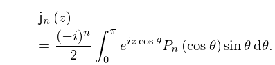
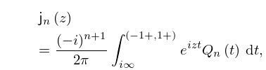
… ►For the Legendre polynomial $P_n$ and the associated Legendre function $Q_n$ see §§18.3 and 14.21(i), with $\mu =0$ and $\nu =n$. …

15: 18.17 Integrals

§18.17 Integrals

… ►

§18.17(v) Fourier Transforms

… ►

§18.17(vi) Laplace Transforms

… ►

§18.17(vii) Mellin Transforms

… ►

§18.17(ix) Compendia

…

16: 18.3 Definitions

§18.3 Definitions

… ►

As given by a Rodrigues formula (18.5.5).

►Table 18.3.1 provides the traditional definitions of Jacobi, Laguerre, and Hermite polynomials via orthogonality and standardization (§§18.2(i) and 18.2(iii)). … ►For explicit power series coefficients up to $n=12$ for these polynomials and for coefficients up to $n=6$ for Jacobi and ultraspherical polynomials see Abramowitz and Stegun (1964, pp. 793–801). … ►For $\nu \in ℝ$ and $N>-\frac{1}{2}$ a finite system of Jacobi polynomials $P_n^{(-N-1+\mathrm{i}\nu ,-N-1-\mathrm{i}\nu )}\left(\mathrm{i}x\right)$ (called pseudo Jacobi polynomials or Routh–Romanovski polynomials) is orthogonal on $(-\mathrm{\infty },\mathrm{\infty })$ with $w(x)={\left(1+x^2\right)}^{-N-1}{\mathrm{e}}^{2\nu \arctan x}$. …

17: 31.9 Orthogonality

§31.9 Orthogonality

►

§31.9(i) Single Orthogonality

… ►The right-hand side may be evaluated at any convenient value, or limiting value, of $\zeta$ in $(0,1)$ since it is independent of $\zeta$. ►For corresponding orthogonality relations for Heun functions (§31.4) and Heun polynomials (§31.5), see Lambe and Ward (1934), Erdélyi (1944), Sleeman (1966a), and Ronveaux (1995, Part A, pp. 59–64). ►

§31.9(ii) Double Orthogonality

…

18: 18.28 Askey–Wilson Class

§18.28 Askey–Wilson Class

… ► … ►

§18.28(ii) Askey–Wilson Polynomials

… ►

Orthogonality

… ►

§18.28(viii) $q$-Racah Polynomials

…

19: 15.9 Relations to Other Functions

… ►

§15.9(i) Orthogonal Polynomials

… ►

Jacobi

… ►

Legendre

… ►

Krawtchouk

… ►

Meixner

…

20: 18.10 Integral Representations

§18.10 Integral Representations

… ►

Ultraspherical

… ►

Legendre

… ►

Jacobi

… ►See also §18.17.