picture

SearchAdvancedHelp

(0.001 seconds)

7 matching pages

1: 36.3 Visualizations of Canonical Integrals

… ►

…

Figure 36.3.1: Modulus of Pearcey integral $|{\mathrm{\Psi }}_2\left(x,y\right)|$.

►

…

Figure 36.3.2: Modulus of swallowtail canonical integral function $|{\mathrm{\Psi }}_3\left(x,y,3\right)|$.

►

…

Figure 36.3.3: Modulus of swallowtail canonical integral function $|{\mathrm{\Psi }}_3\left(x,y,0\right)|$.

►

…

Figure 36.3.4: Modulus of swallowtail canonical integral function $|{\mathrm{\Psi }}_3\left(x,y,-3\right)|$.

… ►

…

Figure 36.3.13: Phase of Pearcey integral $\mathrm{ph}{\mathrm{\Psi }}_2\left(x,y\right)$.

…

2: Sidebar 9.SB1: Supernumerary Rainbows

… ►Airy invented his function in 1838 precisely to describe this phenomenon more accurately than Young had done in 1800 when pointing out that supernumerary rainbows require the wave theory of light and are impossible to explain with Newton’s picture of light as a stream of independent corpuscles. The house in the picture is Newton’s birthplace. …

3: 36.4 Bifurcation Sets

… ►

§36.4(ii) Visualizations

…

4: 36.5 Stokes Sets

… ►

§36.5(iv) Visualizations

… ►

►►

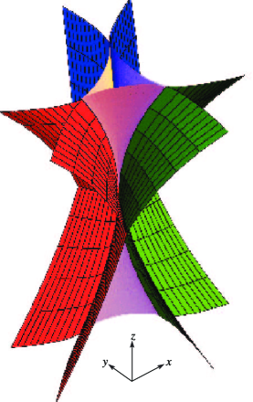
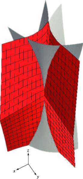
Figure 36.5.8: Sheets of the Stokes surface for the elliptic umbilic catastrophe (colored and with mesh) and the bifurcation set (gray). Magnify

►

►►

Figure 36.5.9: Sheets of the Stokes surface for the hyperbolic umbilic catastrophe (colored and with mesh) and the bifurcation set (gray). Magnify

5: About the Project

… ►These products resulted from the leadership of the Editors and Associate Editors pictured in Figure 1; the contributions of 29 authors, 10 validators, and 5 principal developers; and assistance from a large group of contributing developers, consultants, assistants and interns. …

6: 18.39 Applications in the Physical Sciences

… ►A relativistic treatment becoming necessary as $Z$ becomes large as corrections to the non-relativistic Schrödinger picture are of approximate order ${\left(\alpha Z\right)}^2\sim {\left(Z/137\right)}^2$, $\alpha$ being the dimensionless fine structure constant $e^2/(4\pi {\epsilon }_0\mathrm{\hslash }c)$, where $c$ is the speed of light. …

7: Errata

… ►

Scales were corrected in all figures. The interval $-8.4\le \frac{x-y}{\sqrt{2}}\le 8.4$ was replaced by $-12.0\le \frac{x-y}{\sqrt{2}}\le 12.0$ and $-12.7\le \frac{x+y}{\sqrt{2}}\le 4.2$ replaced by $-18.0\le \frac{x+y}{\sqrt{2}}\le 6.0$. All plots and interactive visualizations were regenerated to improve image quality.

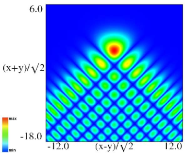
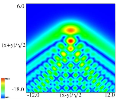
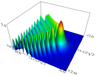
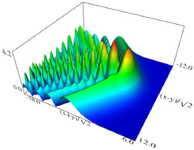
(a) Density plot.	(b) 3D plot.

Figure 36.3.9: Modulus of hyperbolic umbilic canonical integral function $|{\mathrm{\Psi }}^{(\mathrm{H})}\left(x,y,0\right)|$.

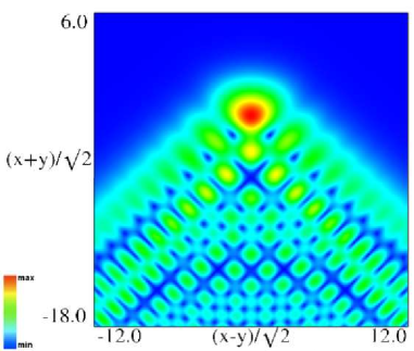
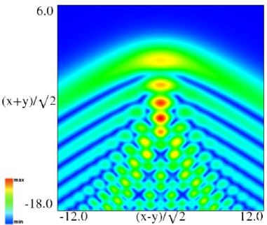
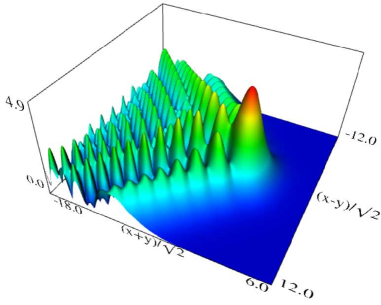
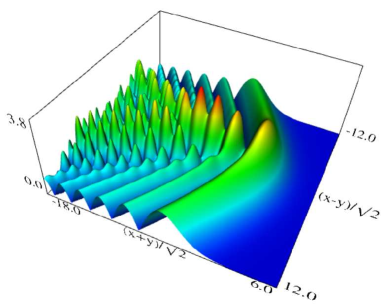
(a) Density plot.	(b) 3D plot.

Figure 36.3.10: Modulus of hyperbolic umbilic canonical integral function $|{\mathrm{\Psi }}^{(\mathrm{H})}\left(x,y,1\right)|$.

(a) Density plot.	(b) 3D plot.

Figure 36.3.11: Modulus of hyperbolic umbilic canonical integral function $|{\mathrm{\Psi }}^{(\mathrm{H})}\left(x,y,2\right)|$.

(a) Density plot.	(b) 3D plot.

Figure 36.3.12: Modulus of hyperbolic umbilic canonical integral function $|{\mathrm{\Psi }}^{(\mathrm{H})}\left(x,y,3\right)|$.

Reported 2016-09-12 by Dan Piponi.

…