phase%20principle

SearchAdvancedHelp

(0.003 seconds)

1—10 of 266 matching pages

1: 3.8 Nonlinear Equations

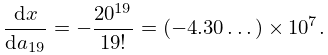
… ►Initial approximations to the zeros can often be found from asymptotic or other approximations to $f(z)$, or by application of the phase principle or Rouché’s theorem; see §1.10(iv). … ►

3.8.15 $$p(x)=(x-1)(x-2)\mathrm{\cdots }(x-20)$$

ⓘ

Permalink:

http://dlmf.nist.gov/3.8.E15

Encodings:

pMML, png, TeX

See also:

Annotations for §3.8(vi), §3.8(vi), §3.8 and Ch.3

… ►Consider $x=20$ and $j=19$. We have $p^{\prime }(20)=19!$ and $a_{19}=1+2+\mathrm{\cdots }+20=210$. … ►

3.8.16 $$\frac{dx}{d{a}_{19}}=-\frac{{20}^{19}}{19!}=(-4.30\mathrm{\dots })\times {10}^7.$$

ⓘ

Symbols:

$\frac{df}{dx}$: derivative of $f$ with respect to $x$ and $!$: factorial (as in $n!$)

Permalink:

http://dlmf.nist.gov/3.8.E16

Encodings:

pMML, png, TeX

See also:

Annotations for §3.8(vi), §3.8(vi), §3.8 and Ch.3

…

2: Bibliography R

… ►

On the definition and properties of generalized $6$-$j$ symbols. J. Math. Phys. 20 (12), pp. 2398–2415.

ⓘ

External Links:

ISSN 0022-2488, Document, MathReview (S. Saran), ZentralBlatt

Referenced by:

§16.4(iii), §16.4(iii).

Encodings:

BibTeX

… ►

Principles of Mathematical Analysis. 3rd edition, McGraw-Hill Book Co., New York.

ⓘ

Notes:

International Series in Pure and Applied Mathematics

External Links:

MathReview, ZentralBlatt

Referenced by:

§1.4(iii).

Encodings:

BibTeX

… ►

On Simple Waves with Profiles in the form of some Special Functions—Chebyshev-Hermite, Mathieu, Whittaker—in Two-phase Media. In Differential Operators and Related Topics, Vol. I (Odessa, 1997), Operator Theory: Advances and Applications, Vol. 117, pp. 313–322.

ⓘ

External Links:

ISBN 3-7643-6287-1, MathReview Entry, ZentralBlatt

Referenced by:

5th item.

Encodings:

BibTeX

…

3: 1.10 Functions of a Complex Variable

… ►

Schwarz Reflection Principle

… ►

Phase (or Argument) Principle

… ►

§1.10(v) Maximum-Modulus Principle

►

Analytic Functions

… ►

Harmonic Functions

…

4: Sidebar 21.SB2: A two-phase solution of the Kadomtsev–Petviashvili equation (21.9.3)

Sidebar 21.SB2: A two-phase solution of the Kadomtsev–Petviashvili equation (21.9.3)

… ►A two-phase solution of the Kadomtsev–Petviashvili equation (21.9.3). Such a solution is given in terms of a Riemann theta function with two phases. …

5: 33.25 Approximations

§33.25 Approximations

►Cody and Hillstrom (1970) provides rational approximations of the phase shift ${\sigma }_0\left(\eta \right)=\mathrm{ph}\mathrm{\Gamma }\left(1+\mathrm{i}\eta \right)$ (see (33.2.10)) for the ranges $0\le \eta \le 2$, $2\le \eta \le 4$, and $4\le \eta \le \mathrm{\infty }$. …

6: 11.6 Asymptotic Expansions

… ►

11.6.1 $${𝐊}_{\nu }\left(z\right)\sim \frac{1}{\pi }\sum _{k=0}^{\mathrm{\infty }}\frac{\mathrm{\Gamma }\left(k+\frac{1}{2}\right){(\frac{1}{2}z)}^{\nu -2k-1}}{\mathrm{\Gamma }\left(\nu +\frac{1}{2}-k\right)},$$ $|\mathrm{ph}z|\le \pi -\delta$,

ⓘ

Symbols:

$\mathrm{\Gamma }\left(z\right)$: gamma function, ${𝐊}_{\nu }\left(z\right)$: Struve function, $\sim$: Poincaré asymptotic expansion, $\pi$: the ratio of the circumference of a circle to its diameter, $\mathrm{ph}$: phase, $z$: complex variable, $\nu$: real or complex order, $k$: nonnegative integer and $\delta$: arbitrary small positive constant

A&S Ref:

12.1.29

Referenced by:

§11.6(i), §11.6(i), §11.6(i), §11.6(i)

Permalink:

http://dlmf.nist.gov/11.6.E1

Encodings:

pMML, png, TeX

See also:

Annotations for §11.6(i), §11.6 and Ch.11

… ►

11.6.2 $${𝐌}_{\nu }\left(z\right)\sim \frac{1}{\pi }\sum _{k=0}^{\mathrm{\infty }}{(-1)}^{k+1}\frac{\mathrm{\Gamma }\left(k+\frac{1}{2}\right){(\frac{1}{2}z)}^{\nu -2k-1}}{\mathrm{\Gamma }\left(\nu +\frac{1}{2}-k\right)},$$ $|\mathrm{ph}z|\le \frac{1}{2}\pi -\delta$.

ⓘ

Symbols:

$\mathrm{\Gamma }\left(z\right)$: gamma function, ${𝐌}_{\nu }\left(z\right)$: modified Struve function, $\sim$: Poincaré asymptotic expansion, $\pi$: the ratio of the circumference of a circle to its diameter, $\mathrm{ph}$: phase, $z$: complex variable, $\nu$: real or complex order, $k$: nonnegative integer and $\delta$: arbitrary small positive constant

A&S Ref:

12.2.6

Referenced by:

§11.6(i), §11.6(i), §11.6(i)

Permalink:

http://dlmf.nist.gov/11.6.E2

Encodings:

pMML, png, TeX

See also:

Annotations for §11.6(i), §11.6 and Ch.11

… ►

11.6.5 $${𝐇}_{\nu }\left(z\right),{𝐋}_{\nu }\left(z\right)\sim \frac{z}{\pi \nu \sqrt{2}}{\left(\frac{\mathrm{e}z}{2\nu }\right)}^{\nu },$$ $|\mathrm{ph}\nu |\le \pi -\delta$.

ⓘ

Symbols:

${𝐇}_{\nu }\left(z\right)$: Struve function, $\sim$: asymptotic equality, $\pi$: the ratio of the circumference of a circle to its diameter, $\mathrm{e}$: base of natural logarithm, ${𝐋}_{\nu }\left(z\right)$: modified Struve function, $\mathrm{ph}$: phase, $z$: complex variable, $\nu$: real or complex order and $\delta$: arbitrary small positive constant

Referenced by:

(11.11.7)

Permalink:

http://dlmf.nist.gov/11.6.E5

Encodings:

pMML, png, TeX

See also:

Annotations for §11.6(ii), §11.6 and Ch.11

… ►

$c_3(\lambda )=20{\lambda }^{-6}-4{\lambda }^{-4},$

… ►

11.6.9 $${𝐋}_{\nu }\left(\lambda \nu \right)\sim I_{\nu }\left(\lambda \nu \right),$$ $|\mathrm{ph}\nu |\le \frac{1}{2}\pi -\delta$,

ⓘ

Symbols:

$\sim$: asymptotic equality, $\pi$: the ratio of the circumference of a circle to its diameter, $I_{\nu }\left(z\right)$: modified Bessel function of the first kind, ${𝐋}_{\nu }\left(z\right)$: modified Struve function, $\mathrm{ph}$: phase, $\nu$: real or complex order, $\delta$: arbitrary small positive constant and $\lambda$: parameter

Referenced by:

§11.6(iii)

Permalink:

http://dlmf.nist.gov/11.6.E9

Encodings:

pMML, png, TeX

See also:

Annotations for §11.6(iii), §11.6 and Ch.11

…

7: 10.3 Graphics

… ►

§10.3(i) Real Order and Variable

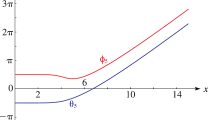
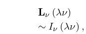
►For the modulus and phase functions $M_{\nu }\left(x\right)$, ${\theta }_{\nu }\left(x\right)$, $N_{\nu }\left(x\right)$, and ${\varphi }_{\nu }\left(x\right)$ see §10.18. … ►

►►

Figure 10.3.4: ${\theta }_5\left(x\right)$, ${\varphi }_5\left(x\right)$, $0\le x\le 15$. Magnify

… ►In the graphics shown in this subsection, height corresponds to the absolute value of the function and color to the phase. …

8: 10.75 Tables

… ►

The main tables in Abramowitz and Stegun (1964, Chapter 9) give $J_0\left(x\right)$ to 15D, $J_1\left(x\right)$, $J_2\left(x\right)$, $Y_0\left(x\right)$, $Y_1\left(x\right)$ to 10D, $Y_2\left(x\right)$ to 8D, $x=0(.1)17.5$; $Y_n\left(x\right)-(2/\pi )J_n\left(x\right)\ln x$, $n=0,1$, $x=0(.1)2$, 8D; $J_n\left(x\right)$, $Y_n\left(x\right)$, $n=3(1)9$, $x=0(.2)20$, 5D or 5S; $J_n\left(x\right)$, $Y_n\left(x\right)$, $n=0(1)20(10)50,100$, $x=1,2,5,10,50,100$, 10S; modulus and phase functions $\sqrt{x}{M}_n\left(x\right)$, ${\theta }_n\left(x\right)-x$, $n=0,1,2$, $1/x=0(.01)0.1$, 8D.

… ►

Bickley et al. (1952) tabulates $x^{-n}{I}_n\left(x\right)$ or ${\mathrm{e}}^{-x}{I}_n\left(x\right)$, $x^n{K}_n\left(x\right)$ or ${\mathrm{e}}^x{K}_n\left(x\right)$, $n=2(1)20$, $x=0$(.01 or .1) 10(.1) 20, 8S; $I_n\left(x\right)$, $K_n\left(x\right)$, $n=0(1)20$, $x=0$ or $0.1(.1)20$, 10S.

… ►

Kerimov and Skorokhodov (1984c) tabulates all zeros of $I_{-n-\frac{1}{2}}\left(z\right)$ and $I_{-n-\frac{1}{2}}^{\prime }\left(z\right)$ in the sector $0\le \mathrm{ph}z\le \frac{1}{2}\pi$ for $n=1(1)20$, 9S.

… ►

Young and Kirk (1964) tabulates ${\mathrm{ber}}_{n}x$, ${\mathrm{bei}}_{n}x$, ${\ker }_{n}x$, ${\mathrm{kei}}_{n}x$, $n=0,1$, $x=0(.1)10$, 15D; ${\mathrm{ber}}_{n}x$, ${\mathrm{bei}}_{n}x$, ${\ker }_{n}x$, ${\mathrm{kei}}_{n}x$, modulus and phase functions $M_n\left(x\right)$, ${\theta }_n\left(x\right)$, $N_n\left(x\right)$, ${\varphi }_n\left(x\right)$, $n=0,1,2$, $x=0(.01)2.5$, 8S, and $n=0(1)10$, $x=0(.1)10$, 7S. Also included are auxiliary functions to facilitate interpolation of the tables for $n=0(1)10$ for small values of $x$. (Concerning the phase functions see §10.68(iv).)

►

Abramowitz and Stegun (1964, Chapter 9) tabulates ${\mathrm{ber}}_{n}x$, ${\mathrm{bei}}_{n}x$, ${\ker }_{n}x$, ${\mathrm{kei}}_{n}x$, $n=0,1$, $x=0(.1)5$, 9–10D; $x^n({\ker }_{n}x+({\mathrm{ber}}_{n}x)(\ln x))$, $x^n({\mathrm{kei}}_{n}x+({\mathrm{bei}}_{n}x)(\ln x))$, $n=0,1$, $x=0(.1)1$, 9D; modulus and phase functions $M_n\left(x\right)$, ${\theta }_n\left(x\right)$, $N_n\left(x\right)$, ${\varphi }_n\left(x\right)$, $n=0,1$, $x=0(.2)7$, 6D; $\sqrt{x}{\mathrm{e}}^{-x/\sqrt{2}}{M}_n\left(x\right)$, ${\theta }_n\left(x\right)-(x/\sqrt{2})$, $\sqrt{x}{\mathrm{e}}^{x/\sqrt{2}}{N}_n\left(x\right)$, ${\varphi }_n\left(x\right)+(x/\sqrt{2})$, $n=0,1$, $1/x=0(.01)0.15$, 5D.

…

9: Bibliography B

… ►

Pionic atoms. Annual Review of Nuclear and Particle Science 20, pp. 467–508.

ⓘ

External Links:

Document

Referenced by:

§33.22(iv).

Encodings:

BibTeX

… ►

Coulomb functions (negative energies). Comput. Phys. Comm. 20 (3), pp. 447–458.

ⓘ

Notes:

Double-precision Fortran code.

External Links:

Document, Code

Referenced by:

1st item, 4th item.

Encodings:

BibTeX

… ►

Phase-space projection identities for diffraction catastrophes. J. Phys. A 13 (1), pp. 149–160.

ⓘ

External Links:

ISSN 0305-4470, Document, MathReview (J. S. Joel), ZentralBlatt

Referenced by:

§36.9.

Encodings:

BibTeX

… ►

Principles of Optics: Electromagnetic Theory of Propagation, Interference and Diffraction of Light. 7th edition, Cambridge University Press, Cambridge.

ⓘ

External Links:

ISBN 0-521-64222-1

Referenced by:

§7.21.

Encodings:

BibTeX

… ►

The determination of phases and amplitudes of wave functions. Proc. Phys. Soc. 81 (3), pp. 442–452.

ⓘ

External Links:

Document

Referenced by:

§33.23(vii).

Encodings:

BibTeX

…

10: 9.7 Asymptotic Expansions

… ►Numerical values of $\chi (n)$ are given in Table 9.7.1 for $n=1(1)20$ to 2D. … ►

9.7.5 $$\mathrm{Ai}\left(z\right)\sim \frac{{\mathrm{e}}^{-\zeta }}{2\sqrt{\pi }{z}^{1/4}}\sum _{k=0}^{\mathrm{\infty }}{(-1)}^k\frac{u_k}{{\zeta }^k},$$ $|\mathrm{ph}z|\le \pi -\delta$,

ⓘ

Symbols:

$\mathrm{Ai}\left(z\right)$: Airy function, $\sim$: Poincaré asymptotic expansion, $\pi$: the ratio of the circumference of a circle to its diameter, $\mathrm{e}$: base of natural logarithm, $\mathrm{ph}$: phase, $k$: nonnegative integer, $z$: complex variable, $\delta$: small positive constant, $\zeta$: change of variable and $u_s$: expansion coefficient

Source:

Olver (1997b, (1.07), pp. 392 and 413)

Referenced by:

(9.10.4), (9.10.6), §9.7(iii), §9.7(iv), §9.7(iv), §9.7(v), Erratum (V1.0.17) for Subsection 9.7(iv)

Permalink:

http://dlmf.nist.gov/9.7.E5

Encodings:

pMML, png, TeX

See also:

Annotations for §9.7(ii), §9.7 and Ch.9

►

9.7.6 $${\mathrm{Ai}}^{\prime }\left(z\right)\sim -\frac{z^{1/4}{\mathrm{e}}^{-\zeta }}{2\sqrt{\pi }}\sum _{k=0}^{\mathrm{\infty }}{(-1)}^k\frac{v_k}{{\zeta }^k},$$ $|\mathrm{ph}z|\le \pi -\delta$,

ⓘ

Symbols:

$\mathrm{Ai}\left(z\right)$: Airy function, $\sim$: Poincaré asymptotic expansion, $\pi$: the ratio of the circumference of a circle to its diameter, $\mathrm{e}$: base of natural logarithm, $\mathrm{ph}$: phase, $k$: nonnegative integer, $z$: complex variable, $\delta$: small positive constant, $\zeta$: change of variable and $v_s$: expansion coefficient

Source:

Olver (1997b, (1.07), pp. 392 and 413)

Referenced by:

§9.7(iii), §9.7(iv), §9.7(iv), §9.7(v), Erratum (V1.0.17) for Subsection 9.7(iv)

Permalink:

http://dlmf.nist.gov/9.7.E6

Encodings:

pMML, png, TeX

See also:

Annotations for §9.7(ii), §9.7 and Ch.9

►

9.7.7 $$\mathrm{Bi}\left(z\right)\sim \frac{{\mathrm{e}}^{\zeta }}{\sqrt{\pi }{z}^{1/4}}\sum _{k=0}^{\mathrm{\infty }}\frac{u_k}{{\zeta }^k},$$ $|\mathrm{ph}z|\le \frac{1}{3}\pi -\delta$,

ⓘ

Symbols:

$\mathrm{Bi}\left(z\right)$: Airy function, $\sim$: Poincaré asymptotic expansion, $\pi$: the ratio of the circumference of a circle to its diameter, $\mathrm{e}$: base of natural logarithm, $\mathrm{ph}$: phase, $k$: nonnegative integer, $z$: complex variable, $\delta$: small positive constant, $\zeta$: change of variable and $u_s$: expansion coefficient

Source:

Olver (1997b, (1.16), pp. 393 and 414)

Referenced by:

(9.10.5), (9.10.7), §9.7(iii), §9.7(iii), §9.7(iv), §9.7(v), Erratum (V1.0.17) for Subsection 9.7(iii)

Permalink:

http://dlmf.nist.gov/9.7.E7

Encodings:

pMML, png, TeX

See also:

Annotations for §9.7(ii), §9.7 and Ch.9

… ►

9.7.17

ⓘ

Symbols:

$\pi$: the ratio of the circumference of a circle to its diameter, $\csc z$: cosecant function, $\cos z$: cosine function, $\exp z$: exponential function, $\mathrm{ph}$: phase, $\mathrm{\Re }$: real part, $z$: complex variable, $\zeta$: change of variable, $\chi (x)$: function, $n$: index and $\sigma$: real variable

Proof sketch:

Derivable from (9.6.1)–(9.6.5) and Nemes (2017b, (26) and Propositions B.1, B.3, B.4).

Referenced by:

§9.7(iv), Erratum (V1.0.11) for Equation (9.7.17)

Permalink:

http://dlmf.nist.gov/9.7.E17

Encodings:

pMML, png, TeX

Modification (effective with 1.0.17):

The bounds have been sharpened for $|\mathrm{ph}z|\le \frac{1}{3}\pi$, from $2\exp \left({\displaystyle \frac{\sigma }{36|\zeta |}}\right)$ to $1$; for $\frac{1}{3}\pi \le |\mathrm{ph}z|\le \frac{2}{3}\pi$, from $2\chi (n)\exp \left({\displaystyle \frac{\sigma \pi }{72|\zeta |}}\right)$ to $\min (|\csc \left(\mathrm{ph}\zeta \right)|,\chi (n+\sigma )+1)$; and for from ${\displaystyle \frac{4\chi (n)}{{|\cos \left(\mathrm{ph}\zeta \right)|}^n}}\exp \left({\displaystyle \frac{\sigma \pi }{36|\mathrm{\Re }\zeta |}}\right)$ to $\frac{\sqrt{2\pi (n+\sigma )}}{{|\cos \left(\mathrm{ph}\zeta \right)|}^{n+\sigma }}+\chi (n+\sigma )+1$.

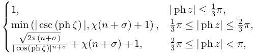
Errata (effective with 1.0.11):

Originally the constraint condition was written incorrectly as $\frac{2}{3}\pi \le |\mathrm{ph}z|\le \pi$. Also, the equation was reformatted to display the constraints in the equation instead of in the text.

Reported 2014-11-05 by Gergő Nemes

See also:

Annotations for §9.7(iv), §9.7 and Ch.9

…