particular solutions

SearchAdvancedHelp

(0.001 seconds)

11—20 of 20 matching pages

11: 28.33 Physical Applications

… ►

Boundary-values problems arising from solution of the two-dimensional wave equation in elliptical coordinates. This yields a pair of equations of the form (28.2.1) and (28.20.1), and the appropriate solution of (28.2.1) is usually a periodic solution of integer order. See §28.33(ii).

… ►The wave equation …The general solution of the problem is a superposition of the separated solutions. … ►In particular, the equation is stable for all sufficiently large values of $\omega$. … ►However, in response to a small perturbation at least one solution may become unbounded. …

12: Mathematical Introduction

… ►Particular care is taken with topics that are not dealt with sufficiently thoroughly from the standpoint of this Handbook in the available literature. These include, for example, multivalued functions of complex variables, for which new definitions of branch points and principal values are supplied (§§1.10(vi), 4.2(i)); the Dirac delta (or delta function), which is introduced in a more readily comprehensible way for mathematicians (§1.17); numerically satisfactory solutions of differential and difference equations (§§2.7(iv), 2.9(i)); and numerical analysis for complex variables (Chapter 3). …

13: Bibliography M

… ►

The 192 solutions of the Heun equation. Math. Comp. 76 (258), pp. 811–843.

ⓘ

External Links:

ISSN 0025-5718, Document, MathReview (Wadim Zudilin), ZentralBlatt (Masaaki Yoshida)

Referenced by:

§31.3(iii).

Encodings:

BibTeX

… ►

Rational solutions of the Painlevé VI equation. J. Phys. A 34 (11), pp. 2281–2294.

ⓘ

External Links:

ISSN 0305-4470, Document, MathReview (Shun Shimomura), ZentralBlatt

Referenced by:

§32.8(vi).

Encodings:

BibTeX

►

Picard and Chazy solutions to the Painlevé VI equation. Math. Ann. 321 (1), pp. 157–195.

ⓘ

External Links:

ISSN 0025-5831, Document, MathReview, ZentralBlatt

Referenced by:

§32.9(iii).

Encodings:

BibTeX

… ►

The accurate evaluation of a particular Fermi-Dirac integral. Comput. Phys. Comm. 101 (1-2), pp. 47–53.

ⓘ

External Links:

Document, ZentralBlatt

Referenced by:

§25.18(i).

Encodings:

BibTeX

… ►

Classical solutions of the third Painlevé equation. Nagoya Math. J. 139, pp. 37–65.

ⓘ

External Links:

ISSN 0027-7630, MathReview (Andrei A. Kapaev), ZentralBlatt

Referenced by:

§32.8(iii).

Encodings:

BibTeX

…

14: 2.11 Remainder Terms; Stokes Phenomenon

… ►In particular, … ►In particular, on the ray $\theta =\pi$ greatest accuracy is achieved by (a) taking the average of the expansions (2.11.6) and (2.11.7), followed by (b) taking account of the exponentially-small contributions arising from the terms involving $h_{2s}(\theta ,\alpha )$ in (2.11.15). … ►

§2.11(v) Exponentially-Improved Expansions (continued)

… ►

2.11.19 $$w_j(z)={\mathrm{e}}^{{\lambda }_{j}z}{z}^{{\mu }_j}\sum _{s=0}^{n-1}\frac{a_{s,j}}{z^s}+R_n^{(j)}(z),$$ $j=1,2$,

ⓘ

Symbols:

$\mathrm{e}$: base of natural logarithm, $R_n^{(j)}(z)$: remainder, $a_{s,j}$: coefficients, ${\lambda }_j$: roots, ${\mu }_j$: quantities and $w_j(z)$: solutions

Permalink:

http://dlmf.nist.gov/2.11.E19

Encodings:

pMML, png, TeX

See also:

Annotations for §2.11(v), §2.11 and Ch.2

…

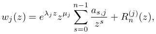
15: 28.28 Integrals, Integral Representations, and Integral Equations

… ►

28.28.1 $$w=\cosh z\cos t\cos \alpha +\sinh z\sin t\sin \alpha .$$

ⓘ

Symbols:

$\cos z$: cosine function, $\cosh z$: hyperbolic cosine function, $\sinh z$: hyperbolic sine function, $\sin z$: sine function, $z$: complex variable, $w(z)$: Mathieu’s equation solution and $\alpha$: parameter

Permalink:

http://dlmf.nist.gov/28.28.E1

Encodings:

pMML, png, TeX

See also:

Annotations for §28.28(i), §28.28 and Ch.28

… ►

28.28.2 $$\frac{1}{2\pi }{\int }_0^{2\pi }{\mathrm{e}}^{2\mathrm{i}hw}{\mathrm{ce}}_n(t,h^2)dt={\mathrm{i}}^n{\mathrm{ce}}_n(\alpha ,h^2){\mathrm{Mc}}_n^{(1)}(z,h),$$

ⓘ

Symbols:

${\mathrm{ce}}_n(z,q)$: Mathieu function, $\pi$: the ratio of the circumference of a circle to its diameter, $dx$: differential of $x$ , $\mathrm{e}$: base of natural logarithm, $\mathrm{i}$: imaginary unit, $\int$: integral, ${\mathrm{Mc}}_n^{(j)}(z,h)$: radial Mathieu function, $h$: parameter, $n$: integer, $z$: complex variable, $w(z)$: Mathieu’s equation solution and $\alpha$: parameter

A&S Ref:

20.7.34 20.7.35 20.7.36 20.7.37

Permalink:

http://dlmf.nist.gov/28.28.E2

Encodings:

pMML, png, TeX

See also:

Annotations for §28.28(i), §28.28 and Ch.28

►

28.28.3 $$\frac{1}{2\pi }{\int }_0^{2\pi }{\mathrm{e}}^{2\mathrm{i}hw}{\mathrm{se}}_n(t,h^2)dt={\mathrm{i}}^n{\mathrm{se}}_n(\alpha ,h^2){\mathrm{Ms}}_n^{(1)}(z,h),$$

ⓘ

Symbols:

${\mathrm{se}}_n(z,q)$: Mathieu function, $\pi$: the ratio of the circumference of a circle to its diameter, $dx$: differential of $x$ , $\mathrm{e}$: base of natural logarithm, $\mathrm{i}$: imaginary unit, $\int$: integral, ${\mathrm{Ms}}_n^{(j)}(z,h)$: radial Mathieu function, $h$: parameter, $n$: integer, $z$: complex variable, $w(z)$: Mathieu’s equation solution and $\alpha$: parameter

Permalink:

http://dlmf.nist.gov/28.28.E3

Encodings:

pMML, png, TeX

See also:

Annotations for §28.28(i), §28.28 and Ch.28

… ►In particular, when $h>0$ the integrals (28.28.11), (28.28.14) converge absolutely and uniformly in the half strip $\mathrm{\Re }z\ge 0$, $0\le \mathrm{\Im }z\le \pi$. … ►In particular, for integer $\nu$ and $\mathrm{\ell }=0,1,2,\mathrm{\dots }$, …

16: 14.19 Toroidal (or Ring) Functions

… ►When $\nu =n-\frac{1}{2}$, $n=0,1,2,\mathrm{\dots }$, $\mu \in ℝ$, and $x\in (1,\mathrm{\infty })$ solutions of (14.2.2) are known as toroidal or ring functions. …In particular, for $\mu =0$ and $\nu =\pm \frac{1}{2}$ see §14.5(v). …

17: 3.8 Nonlinear Equations

§3.8 Nonlinear Equations

… ►Solutions are called roots of the equation, or zeros of $f$. … ►and the solutions are called fixed points of $\varphi$. … ►For describing the distribution of complex zeros of solutions of linear homogeneous second-order differential equations by methods based on the Liouville–Green (WKB) approximation, see Segura (2013). … ►For an arbitrary starting point $z_0\in ℂ$, convergence cannot be predicted, and the boundary of the set of points $z_0$ that generate a sequence converging to a particular zero has a very complicated structure. …

18: 13.2 Definitions and Basic Properties

… ►

Standard Solutions

►The first two standard solutions are: … ►In particular, … ►

§13.2(v) Numerically Satisfactory Solutions

… ► …

19: 15.2 Definitions and Analytical Properties

… ►In particular … ►(Both interpretations give solutions of the hypergeometric differential equation (15.10.1), as does $𝐅(a,b;c;z)$, which is analytic at $c=0,-1,-2,\mathrm{\dots }$.) …

20: 1.18 Linear Second Order Differential Operators and Eigenfunction Expansions

… ►This question may be rephrased by asking: do $f(x)$ and $g(x)$ satisfy the same boundary conditions which are needed to fully specify the solutions of a second order linear differential equation? A simple example is the choice $f(a)=f(b)=0$, and $g(a)=g(b)=0$, this being only one of many. … ►In particular, this holds for $F(\lambda )={\left(z-\lambda \right)}^{-1}$, $z\in ℂ\setminus {𝝈}_c$ … ►Then, for $z\in ℂ\backslash ℝ$, $f\in N_z$ iff $f$ is an ordinary solution (i. … ►See, in particular, the overview Everitt (2005b, pp. 45–74), and the uniformly annotated listing of $51$ solved Sturm–Liouville problems in Everitt (2005a, pp. 272–331), each with their limit point, or circle, boundary behaviors categorized.