partial

SearchAdvancedHelp

(0.001 seconds)

11—20 of 95 matching pages

11: 28.32 Mathematical Applications

… ►

28.32.2 $$\frac{{\partial }^{2}V}{{\partial x}^2}+\frac{{\partial }^{2}V}{{\partial y}^2}+k^{2}V=0$$

ⓘ

Symbols:

$\frac{\partial f}{\partial x}$: partial derivative of $f$ with respect to $x$ , $\partial x$: partial differential of $x$ , $x$: real variable, $y$: real variable, $k$: parameter and $V(\xi ,\eta )$: solution

Referenced by:

§28.33(ii)

Permalink:

http://dlmf.nist.gov/28.32.E2

Encodings:

pMML, png, TeX

See also:

Annotations for §28.32(i), §28.32 and Ch.28

… ►

28.32.3 $$\frac{{\partial }^{2}V}{{\partial \xi }^2}+\frac{{\partial }^{2}V}{{\partial \eta }^2}+\frac{1}{2}{c}^2{k}^2(\cosh \left(2\xi \right)-\cos \left(2\eta \right))V=0.$$

ⓘ

Symbols:

$\cos z$: cosine function, $\cosh z$: hyperbolic cosine function, $\frac{\partial f}{\partial x}$: partial derivative of $f$ with respect to $x$ , $\partial x$: partial differential of $x$ , $\eta$: variable, $\xi$: variable, $k$: parameter and $V(\xi ,\eta )$: solution

Referenced by:

§28.32(i), §28.33(ii)

Permalink:

http://dlmf.nist.gov/28.32.E3

Encodings:

pMML, png, TeX

See also:

Annotations for §28.32(i), §28.32 and Ch.28

… ►

28.32.4 $$\frac{{\partial }^{2}K}{{\partial z}^2}-\frac{{\partial }^{2}K}{{\partial \zeta }^2}=2q\left(\cos \left(2z\right)-\cos \left(2\zeta \right)\right)K.$$

ⓘ

Symbols:

$\cos z$: cosine function, $\frac{\partial f}{\partial x}$: partial derivative of $f$ with respect to $x$ , $\partial x$: partial differential of $x$ , $q=h^2$: parameter, $z$: complex variable, $\zeta$: variable and $K(z,\zeta )$: solution

Permalink:

http://dlmf.nist.gov/28.32.E4

Encodings:

pMML, png, TeX

See also:

Annotations for §28.32(i), §28.32 and Ch.28

… ►

28.32.5 $$K(z,\zeta )\frac{du(\zeta )}{d\zeta }-u(\zeta )\frac{\partial K(z,\zeta )}{\partial \zeta }$$

ⓘ

Symbols:

$\frac{df}{dx}$: derivative of $f$ with respect to $x$ , $\frac{\partial f}{\partial x}$: partial derivative of $f$ with respect to $x$ , $\partial x$: partial differential of $x$ , $z$: complex variable, $\zeta$: variable, $u(\zeta )$: solution and $K(z,\zeta )$: solution

Permalink:

http://dlmf.nist.gov/28.32.E5

Encodings:

pMML, png, TeX

See also:

Annotations for §28.32(i), §28.32 and Ch.28

…

12: 20.13 Physical Applications

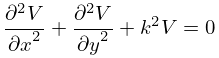
… ►The functions ${\theta }_j\left(z\right|\tau )$, $j=1,2,3,4$, provide periodic solutions of the partial differential equation ►

20.13.1 $$\partial \theta (z|\tau )/\partial \tau =\kappa {\partial }^2\theta (z|\tau )/{\partial z}^2,$$

ⓘ

Symbols:

$\frac{\partial f}{\partial x}$: partial derivative of $f$ with respect to $x$ , $\partial x$: partial differential of $x$ , $\tau$: lattice parameter and $z$: real variable

Referenced by:

§20.13

Permalink:

http://dlmf.nist.gov/20.13.E1

Encodings:

pMML, png, TeX

See also:

Annotations for §20.13 and Ch.20

… ►

20.13.2 $$\partial \theta /\partial t=\alpha {\partial }^2\theta /{\partial z}^2,$$

ⓘ

Symbols:

$\frac{\partial f}{\partial x}$: partial derivative of $f$ with respect to $x$ , $\partial x$: partial differential of $x$ , $t$: time, $\alpha$: real parameter and $z$: real variable

Referenced by:

§20.13

Permalink:

http://dlmf.nist.gov/20.13.E2

Encodings:

pMML, png, TeX

See also:

Annotations for §20.13 and Ch.20

…

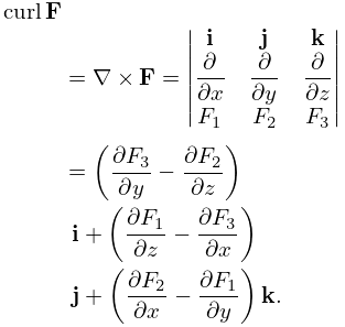
13: 1.6 Vectors and Vector-Valued Functions

… ►

1.6.19 $$\nabla =𝐢\frac{\partial }{\partial x}+𝐣\frac{\partial }{\partial y}+𝐤\frac{\partial }{\partial z}.$$

ⓘ

Symbols:

$\frac{\partial f}{\partial x}$: partial derivative of $f$ with respect to $x$ , $\partial x$: partial differential of $x$ , $z$: variable, $𝐢$: unit vector, $𝐣$: unit vector and $𝐤$: unit vector

Permalink:

http://dlmf.nist.gov/1.6.E19

Encodings:

pMML, png, TeX

See also:

Annotations for §1.6(iii), §1.6(iii), §1.6 and Ch.1

… ►

1.6.20 $$\mathrm{grad}f=\nabla f=\frac{\partial f}{\partial x}𝐢+\frac{\partial f}{\partial y}𝐣+\frac{\partial f}{\partial z}𝐤.$$

ⓘ

Defines:

$\mathrm{grad}$: gradient of differentiable scalar function

Symbols:

$\frac{\partial f}{\partial x}$: partial derivative of $f$ with respect to $x$ , $\partial x$: partial differential of $x$ , $z$: variable, $𝐢$: unit vector, $𝐣$: unit vector and $𝐤$: unit vector

Permalink:

http://dlmf.nist.gov/1.6.E20

Encodings:

pMML, png, TeX

See also:

Annotations for §1.6(iii), §1.6(iii), §1.6 and Ch.1

… ►

1.6.22

ⓘ

Defines:

$\mathrm{curl}$: of vector-valued function

Symbols:

$det$: determinant, $\frac{\partial f}{\partial x}$: partial derivative of $f$ with respect to $x$ , $\partial x$: partial differential of $x$ , $z$: variable, $𝐢$: unit vector, $𝐣$: unit vector, $𝐤$: unit vector and $F_j$: vector function components

Permalink:

http://dlmf.nist.gov/1.6.E22

Encodings:

pMML, png, TeX

See also:

Annotations for §1.6(iii), §1.6(iii), §1.6 and Ch.1

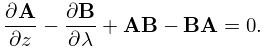
… ►Suppose $S$ is an oriented surface with boundary $\partial S$ which is oriented so that its direction is clockwise relative to the normals of $S$. … ►where $\partial g/\partial n=\nabla g\cdot 𝐧$ is the derivative of $g$ normal to the surface outwards from $V$ and $𝐧$ is the unit outer normal vector. …

14: 3.4 Differentiation

… ►

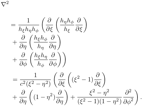
§3.4(iii) Partial Derivatives

… ► … ►The results in this subsection for the partial derivatives follow from Panow (1955, Table 10). Those for the Laplacian and the biharmonic operator follow from the formulas for the partial derivatives. … ►

15: 19.4 Derivatives and Differential Equations

… ►

19.4.4 $$\frac{\partial \mathrm{\Pi }({\alpha }^2,k)}{\partial k}=\frac{k}{k_{}^{\prime }{}_{}{}^2(k^2-{\alpha }^2)}(E\left(k\right)-k_{}^{\prime }{}_{}{}^2\mathrm{\Pi }({\alpha }^2,k)).$$

ⓘ

Symbols:

$E\left(k\right)$: Legendre’s complete elliptic integral of the second kind, $\mathrm{\Pi }({\alpha }^2,k)$: Legendre’s complete elliptic integral of the third kind, $\frac{\partial f}{\partial x}$: partial derivative of $f$ with respect to $x$ , $\partial x$: partial differential of $x$ , $k$: real or complex modulus, $k^{\prime }$: complementary modulus and ${\alpha }^2$: real or complex parameter

Permalink:

http://dlmf.nist.gov/19.4.E4

Encodings:

pMML, png, TeX

See also:

Annotations for §19.4(i), §19.4 and Ch.19

►

19.4.5 $$\frac{\partial F(\varphi ,k)}{\partial k}=\frac{E(\varphi ,k)-k_{}^{\prime }{}_{}{}^{2}F(\varphi ,k)}{kk_{}^{\prime }{}_{}{}^2}-\frac{k\sin \varphi \cos \varphi }{k_{}^{\prime }{}_{}{}^2\sqrt{1-k^2{\sin }^2\varphi }},$$

ⓘ

Symbols:

$\cos z$: cosine function, $F(\varphi ,k)$: Legendre’s incomplete elliptic integral of the first kind, $E(\varphi ,k)$: Legendre’s incomplete elliptic integral of the second kind, $\frac{\partial f}{\partial x}$: partial derivative of $f$ with respect to $x$ , $\partial x$: partial differential of $x$ , $\sin z$: sine function, $\varphi$: real or complex argument, $k$: real or complex modulus and $k^{\prime }$: complementary modulus

Permalink:

http://dlmf.nist.gov/19.4.E5

Encodings:

pMML, png, TeX

See also:

Annotations for §19.4(i), §19.4 and Ch.19

►

19.4.6 $$\frac{\partial E(\varphi ,k)}{\partial k}=\frac{E(\varphi ,k)-F(\varphi ,k)}{k},$$

ⓘ

Symbols:

$F(\varphi ,k)$: Legendre’s incomplete elliptic integral of the first kind, $E(\varphi ,k)$: Legendre’s incomplete elliptic integral of the second kind, $\frac{\partial f}{\partial x}$: partial derivative of $f$ with respect to $x$ , $\partial x$: partial differential of $x$ , $\varphi$: real or complex argument and $k$: real or complex modulus

Referenced by:

§19.30(i)

Permalink:

http://dlmf.nist.gov/19.4.E6

Encodings:

pMML, png, TeX

See also:

Annotations for §19.4(i), §19.4 and Ch.19

►

19.4.7 $$\frac{\partial \mathrm{\Pi }(\varphi ,{\alpha }^2,k)}{\partial k}=\frac{k}{k_{}^{\prime }{}_{}{}^2(k^2-{\alpha }^2)}\left(E(\varphi ,k)-k_{}^{\prime }{}_{}{}^2\mathrm{\Pi }(\varphi ,{\alpha }^2,k)-\frac{k^2\sin \varphi \cos \varphi }{\sqrt{1-k^2{\sin }^2\varphi }}\right).$$

ⓘ

Symbols:

$\cos z$: cosine function, $E(\varphi ,k)$: Legendre’s incomplete elliptic integral of the second kind, $\mathrm{\Pi }(\varphi ,{\alpha }^2,k)$: Legendre’s incomplete elliptic integral of the third kind, $\frac{\partial f}{\partial x}$: partial derivative of $f$ with respect to $x$ , $\partial x$: partial differential of $x$ , $\sin z$: sine function, $\varphi$: real or complex argument, $k$: real or complex modulus, $k^{\prime }$: complementary modulus and ${\alpha }^2$: real or complex parameter

Permalink:

http://dlmf.nist.gov/19.4.E7

Encodings:

pMML, png, TeX

See also:

Annotations for §19.4(i), §19.4 and Ch.19

… ►Let $D_k=\partial /\partial k$. …

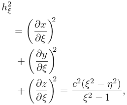
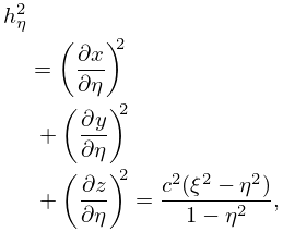
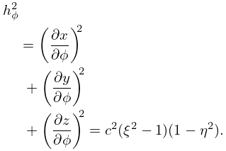
16: 30.13 Wave Equation in Prolate Spheroidal Coordinates

… ►

30.13.3 $$h_{\xi }^2={\left(\frac{\partial x}{\partial \xi }\right)}^2+{\left(\frac{\partial y}{\partial \xi }\right)}^2+{\left(\frac{\partial z}{\partial \xi }\right)}^2=\frac{c^2({\xi }^2-{\eta }^2)}{{\xi }^2-1},$$

ⓘ

Symbols:

$\frac{\partial f}{\partial x}$: partial derivative of $f$ with respect to $x$ , $\partial x$: partial differential of $x$ , $z$: complex variable, $x$: real variable, $y$: real variable, $\xi$: prolate spheroidal coordinate, $\eta$: prolate spheroidal coordinate, $c$: positive constant and $h_{\xi },h_{\eta },h_{\varphi }$: metric coefficients

A&S Ref:

21.4.2

Permalink:

http://dlmf.nist.gov/30.13.E3

Encodings:

pMML, png, TeX

See also:

Annotations for §30.13(ii), §30.13 and Ch.30

►

30.13.4 $$h_{\eta }^2={\left(\frac{\partial x}{\partial \eta }\right)}^2+{\left(\frac{\partial y}{\partial \eta }\right)}^2+{\left(\frac{\partial z}{\partial \eta }\right)}^2=\frac{c^2({\xi }^2-{\eta }^2)}{1-{\eta }^2},$$

ⓘ

Symbols:

$\frac{\partial f}{\partial x}$: partial derivative of $f$ with respect to $x$ , $\partial x$: partial differential of $x$ , $z$: complex variable, $x$: real variable, $y$: real variable, $\xi$: prolate spheroidal coordinate, $\eta$: prolate spheroidal coordinate, $c$: positive constant and $h_{\xi },h_{\eta },h_{\varphi }$: metric coefficients

Permalink:

http://dlmf.nist.gov/30.13.E4

Encodings:

pMML, png, TeX

See also:

Annotations for §30.13(ii), §30.13 and Ch.30

►

30.13.5 $$h_{\varphi }^2={\left(\frac{\partial x}{\partial \varphi }\right)}^2+{\left(\frac{\partial y}{\partial \varphi }\right)}^2+{\left(\frac{\partial z}{\partial \varphi }\right)}^2=c^2({\xi }^2-1)(1-{\eta }^2).$$

ⓘ

Symbols:

$\frac{\partial f}{\partial x}$: partial derivative of $f$ with respect to $x$ , $\partial x$: partial differential of $x$ , $z$: complex variable, $x$: real variable, $y$: real variable, $\xi$: prolate spheroidal coordinate, $\eta$: prolate spheroidal coordinate, $\varphi$: prolate spheroidal coordinate, $c$: positive constant and $h_{\xi },h_{\eta },h_{\varphi }$: metric coefficients

Permalink:

http://dlmf.nist.gov/30.13.E5

Encodings:

pMML, png, TeX

See also:

Annotations for §30.13(ii), §30.13 and Ch.30

… ►

30.13.6 $${\nabla }^2=\frac{1}{h_{\xi }{h}_{\eta }{h}_{\varphi }}\left(\frac{\partial }{\partial \xi }\left(\frac{h_{\eta }{h}_{\varphi }}{h_{\xi }}\frac{\partial }{\partial \xi }\right)+\frac{\partial }{\partial \eta }\left(\frac{h_{\xi }{h}_{\varphi }}{h_{\eta }}\frac{\partial }{\partial \eta }\right)+\frac{\partial }{\partial \varphi }\left(\frac{h_{\xi }{h}_{\eta }}{h_{\varphi }}\frac{\partial }{\partial \varphi }\right)\right)=\frac{1}{c^2({\xi }^2-{\eta }^2)}\left(\frac{\partial }{\partial \xi }\left(({\xi }^2-1)\frac{\partial }{\partial \xi }\right)+\frac{\partial }{\partial \eta }\left((1-{\eta }^2)\frac{\partial }{\partial \eta }\right)+\frac{{\xi }^2-{\eta }^2}{({\xi }^2-1)(1-{\eta }^2)}\frac{{\partial }^2}{{\partial \varphi }^2}\right).$$

ⓘ

Symbols:

$\frac{\partial f}{\partial x}$: partial derivative of $f$ with respect to $x$ , $\partial x$: partial differential of $x$ , $\xi$: prolate spheroidal coordinate, $\eta$: prolate spheroidal coordinate, $\varphi$: prolate spheroidal coordinate, $c$: positive constant and $h_{\xi },h_{\eta },h_{\varphi }$: metric coefficients

A&S Ref:

21.5.1 (in corrected form)

Permalink:

http://dlmf.nist.gov/30.13.E6

Encodings:

pMML, png, TeX

See also:

Annotations for §30.13(iii), §30.13 and Ch.30

…

17: 31.10 Integral Equations and Representations

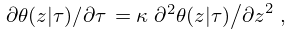
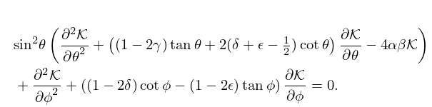
… ►and the kernel $𝒦(z,t)$ is a solution of the partial differential equation … ►

31.10.4 $${𝒟}_z=z(z-1)(z-a)({\partial }^2/{\partial z}^2)+\left(\gamma (z-1)(z-a)+\delta z(z-a)+ϵz(z-1)\right)(\partial /\partial z)+\alpha \beta z.$$

ⓘ

Defines:

${𝒟}_z$: Heun’s operator (locally)

Symbols:

$\frac{\partial f}{\partial x}$: partial derivative of $f$ with respect to $x$ , $\partial x$: partial differential of $x$ , $z$: complex variable, $\gamma$: real or complex parameter, $\delta$: real or complex parameter, $ϵ$: real or complex parameter, $a$: complex parameter, $\alpha$: real or complex parameter and $\beta$: real or complex parameter

Referenced by:

§31.10(ii)

Permalink:

http://dlmf.nist.gov/31.10.E4

Encodings:

pMML, png, TeX

See also:

Annotations for §31.10(i), §31.10 and Ch.31

… ►

31.10.8 $${\sin }^2\theta \left(\frac{{\partial }^2𝒦}{{\partial \theta }^2}+\left((1-2\gamma )\tan \theta +2(\delta +ϵ-\frac{1}{2})\cot \theta \right)\frac{\partial 𝒦}{\partial \theta }-4\alpha \beta 𝒦\right)+\frac{{\partial }^2𝒦}{{\partial \varphi }^2}+\left((1-2\delta )\cot \varphi -(1-2ϵ)\tan \varphi \right)\frac{\partial 𝒦}{\partial \varphi }=0.$$

ⓘ

Symbols:

$\cot z$: cotangent function, $\frac{\partial f}{\partial x}$: partial derivative of $f$ with respect to $x$ , $\partial x$: partial differential of $x$ , $\sin z$: sine function, $\tan z$: tangent function, $\gamma$: real or complex parameter, $\delta$: real or complex parameter, $ϵ$: real or complex parameter, $\alpha$: real or complex parameter, $\beta$: real or complex parameter, $𝒦(z,t)$: kernel, $\theta$: angle and $\varphi$: angle

Referenced by:

§31.10(i)

Permalink:

http://dlmf.nist.gov/31.10.E8

Encodings:

pMML, png, TeX

See also:

Annotations for §31.10(i), §31.10(i), §31.10 and Ch.31

… ►and the kernel $𝒦(z;s,t)$ is a solution of the partial differential equation … ►

31.10.18 $$\frac{{\partial }^2𝒦}{{\partial u}^2}+\frac{{\partial }^2𝒦}{{\partial v}^2}+\frac{{\partial }^2𝒦}{{\partial w}^2}+\frac{2\gamma -1}{u}\frac{\partial 𝒦}{\partial u}+\frac{2\delta -1}{v}\frac{\partial 𝒦}{\partial v}+\frac{2ϵ-1}{w}\frac{\partial 𝒦}{\partial w}=0.$$

ⓘ

Symbols:

$\frac{\partial f}{\partial x}$: partial derivative of $f$ with respect to $x$ , $\partial x$: partial differential of $x$ , $\gamma$: real or complex parameter, $\delta$: real or complex parameter, $ϵ$: real or complex parameter, $𝒦(z;s,t)$: kernel, $u$ , $v$ and $w$

Permalink:

http://dlmf.nist.gov/31.10.E18

Encodings:

pMML, png, TeX

See also:

Annotations for §31.10(ii), §31.10(ii), §31.10 and Ch.31

…

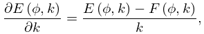
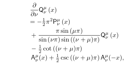
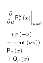
18: 14.11 Derivatives with Respect to Degree or Order

… ►

14.11.1 $$\frac{\partial }{\partial \nu }{𝖯}_{\nu }^{\mu }\left(x\right)=\pi \cot \left(\nu \pi \right){𝖯}_{\nu }^{\mu }\left(x\right)-\frac{1}{\pi }{𝖠}_{\nu }^{\mu }(x),$$

ⓘ

Symbols:

: Ferrers function of the first kind, $\pi$: the ratio of the circumference of a circle to its diameter, $\cot z$: cotangent function, $\frac{\partial f}{\partial x}$: partial derivative of $f$ with respect to $x$ , $\partial x$: partial differential of $x$ , $x$: real variable, $\mu$: general order, $\nu$: general degree and ${𝖠}_{\nu }^{\mu }(x)$

Referenced by:

§14.11, §14.11

Permalink:

http://dlmf.nist.gov/14.11.E1

Encodings:

pMML, png, TeX

See also:

Annotations for §14.11 and Ch.14

►

14.11.2 $$\frac{\partial }{\partial \nu }{𝖰}_{\nu }^{\mu }\left(x\right)=-\frac{1}{2}{\pi }^2{𝖯}_{\nu }^{\mu }\left(x\right)+\frac{\pi \sin \left(\mu \pi \right)}{\sin \left(\nu \pi \right)\sin \left((\nu +\mu )\pi \right)}{𝖰}_{\nu }^{\mu }\left(x\right)-\frac{1}{2}\cot \left((\nu +\mu )\pi \right){𝖠}_{\nu }^{\mu }(x)+\frac{1}{2}\csc \left((\nu +\mu )\pi \right){𝖠}_{\nu }^{\mu }(-x),$$

ⓘ

Symbols:

: Ferrers function of the first kind, : Ferrers function of the second kind, $\pi$: the ratio of the circumference of a circle to its diameter, $\csc z$: cosecant function, $\cot z$: cotangent function, $\frac{\partial f}{\partial x}$: partial derivative of $f$ with respect to $x$ , $\partial x$: partial differential of $x$ , $\sin z$: sine function, $x$: real variable, $\mu$: general order, $\nu$: general degree and ${𝖠}_{\nu }^{\mu }(x)$

Referenced by:

§14.11

Permalink:

http://dlmf.nist.gov/14.11.E2

Encodings:

pMML, png, TeX

See also:

Annotations for §14.11 and Ch.14

… ►

14.11.4 $${\frac{\partial }{\partial \mu }{𝖯}_{\nu }^{\mu }\left(x\right)|}_{\mu =0}=\left(\psi \left(-\nu \right)-\pi \cot \left(\nu \pi \right)\right){𝖯}_{\nu }\left(x\right)+{𝖰}_{\nu }\left(x\right),$$

ⓘ

Symbols:

: Ferrers function of the first kind, $\pi$: the ratio of the circumference of a circle to its diameter, $\cot z$: cotangent function, $\psi \left(z\right)$: psi (or digamma) function, $\frac{\partial f}{\partial x}$: partial derivative of $f$ with respect to $x$ , $\partial x$: partial differential of $x$ , ${𝖯}_{\nu }\left(x\right)={𝖯}_{\nu }^0\left(x\right)$: Ferrers function of the first kind, ${𝖰}_{\nu }\left(x\right)={𝖰}_{\nu }^0\left(x\right)$: Ferrers function of the second kind, $x$: real variable, $\mu$: general order and $\nu$: general degree

Referenced by:

§14.11, §14.11

Permalink:

http://dlmf.nist.gov/14.11.E4

Encodings:

pMML, png, TeX

See also:

Annotations for §14.11 and Ch.14

►

14.11.5 $${\frac{\partial }{\partial \mu }{𝖰}_{\nu }^{\mu }\left(x\right)|}_{\mu =0}=-\frac{1}{4}{\pi }^2{𝖯}_{\nu }\left(x\right)+\left(\psi \left(-\nu \right)-\pi \cot \left(\nu \pi \right)\right){𝖰}_{\nu }\left(x\right).$$

ⓘ

Symbols:

: Ferrers function of the second kind, $\pi$: the ratio of the circumference of a circle to its diameter, $\cot z$: cotangent function, $\psi \left(z\right)$: psi (or digamma) function, $\frac{\partial f}{\partial x}$: partial derivative of $f$ with respect to $x$ , $\partial x$: partial differential of $x$ , ${𝖯}_{\nu }\left(x\right)={𝖯}_{\nu }^0\left(x\right)$: Ferrers function of the first kind, ${𝖰}_{\nu }\left(x\right)={𝖰}_{\nu }^0\left(x\right)$: Ferrers function of the second kind, $x$: real variable, $\mu$: general order and $\nu$: general degree

Referenced by:

§14.11

Permalink:

http://dlmf.nist.gov/14.11.E5

Encodings:

pMML, png, TeX

See also:

Annotations for §14.11 and Ch.14

…

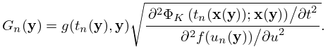
19: 36.12 Uniform Approximation of Integrals

… ►Also, $f$ is real analytic, and ${\partial }^{K+2}f/{\partial u}^{K+2}>0$ for all $𝐲$ such that all $K+1$ critical points coincide. If , then we may evaluate the complex conjugate of $I$ for real values of $𝐲$ and $g$, and obtain $I$ by conjugation and analytic continuation. … ►

36.12.2 $$\frac{\partial }{\partial u}f(u_j(𝐲);𝐲)=0.$$

ⓘ

Symbols:

$\frac{\partial f}{\partial x}$: partial derivative of $f$ with respect to $x$ , $\partial x$: partial differential of $x$ , $f(u,𝐲)$: function and $u(t;𝐲)$: mapping

Permalink:

http://dlmf.nist.gov/36.12.E2

Encodings:

pMML, png, TeX

See also:

Annotations for §36.12(i), §36.12 and Ch.36

… ►

36.12.10 $$G_n(𝐲)=g(t_n(𝐲),𝐲)\sqrt{\frac{{\partial }^2{\mathrm{\Phi }}_K(t_n(𝐱(𝐲));𝐱(𝐲))/{\partial t}^2}{{\partial }^{2}f(u_n(𝐲))/{\partial u}^2}}.$$

ⓘ

Symbols:

${\mathrm{\Phi }}_K(t;𝐱)$: cuspoid catastrophe of codimension $K$ , $\frac{\partial f}{\partial x}$: partial derivative of $f$ with respect to $x$ , $\partial x$: partial differential of $x$ , $m$: integer, $t$: variable, $K$: codimension, $g(u,𝐲)$: function, $f(u,𝐲)$: function, $u(t;𝐲)$: mapping, $𝐱(𝐲)$: function and $t_j(𝐱)$: solutions

Referenced by:

§36.12(i)

Permalink:

http://dlmf.nist.gov/36.12.E10

Encodings:

pMML, png, TeX

See also:

Annotations for §36.12(i), §36.12 and Ch.36

… ►

$f_{\pm }^{\prime \prime }={\displaystyle \frac{{\partial }^2}{{\partial u}^2}}f(u_{\pm }(y),y),$

…

20: 32.4 Isomonodromy Problems

… ►

${\displaystyle \frac{\partial 𝚿}{\partial \lambda }}=𝐀(z,\lambda )𝚿,$

►

${\displaystyle \frac{\partial 𝚿}{\partial z}}=𝐁(z,\lambda )𝚿,$

… ►

32.4.2 $$\frac{{\partial }^2𝚿}{\partial z\partial \lambda }=\frac{{\partial }^2𝚿}{\partial \lambda \partial z},$$

ⓘ

Symbols:

$\partial x$: partial differential of $x$ and $z$: real

Permalink:

http://dlmf.nist.gov/32.4.E2

Encodings:

pMML, png, TeX

See also:

Annotations for §32.4(i), §32.4 and Ch.32

… ►

32.4.3 $$\frac{\partial 𝐀}{\partial z}-\frac{\partial 𝐁}{\partial \lambda }+𝐀𝐁-𝐁𝐀=0.$$

ⓘ

Symbols:

$\frac{\partial f}{\partial x}$: partial derivative of $f$ with respect to $x$ , $\partial x$: partial differential of $x$ and $z$: real

Referenced by:

§32.4(i)

Permalink:

http://dlmf.nist.gov/32.4.E3

Encodings:

pMML, png, TeX

See also:

Annotations for §32.4(i), §32.4 and Ch.32

…