parameter constraint

SearchAdvancedHelp

(0.002 seconds)

1—10 of 22 matching pages

1: 18.3 Definitions

… ►

Table 18.3.1: Orthogonality properties for classical OP’s: intervals, weight functions, standardizations, leading coefficients, and parameter constraints. …For further implications of the parameter constraints see the Note in §18.5(iii).

► ►►

Name	$p_n(x)$	$(a,b)$	$w(x)$	$h_n$	$k_n$	${\tilde{k}}_n/k_n$	Constraints
…

►

…

2: 18.5 Explicit Representations

… ►For corresponding formulas for Chebyshev, Legendre, and the Hermite ${\mathrm{𝐻𝑒}}_n$ polynomials apply (18.7.3)–(18.7.6), (18.7.9), and (18.7.11). … ► …

3: 18.25 Wilson Class: Definitions

… ►Table 18.25.1 lists the transformations of variable, orthogonality ranges, and parameter constraints that are needed in §18.2(i) for the Wilson polynomials $W_n(x;a,b,c,d)$, continuous dual Hahn polynomials $S_n(x;a,b,c)$, Racah polynomials $R_n(x;\alpha ,\beta ,\gamma ,\delta )$, and dual Hahn polynomials $R_n(x;\gamma ,\delta ,N)$. ►

Table 18.25.1: Wilson class OP’s: transformations of variable, orthogonality ranges, and parameter constraints.

► ►►

OP	$p_n(x)$	$x=\lambda (y)$	Orthogonality range for $y$	Constraints
…

►

…

4: 18.19 Hahn Class: Definitions

… ►

Table 18.19.1: Orthogonality properties for Hahn, Krawtchouk, Meixner, and Charlier OP’s: discrete sets, weight functions, standardizations, and parameter constraints.

► ►►

	$p_n(x)$	$X$	$w_x$	$h_n$
…

►

…

5: 20.10 Integrals

… ►

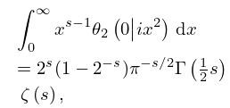
§20.10(i) Mellin Transforms with respect to the Lattice Parameter

►

20.10.1 $${\int }_0^{\mathrm{\infty }}{x}^{s-1}{\theta }_2\left(0\right|\mathrm{i}{x}^2)dx=2^s(1-2^{-s}){\pi }^{-s/2}\mathrm{\Gamma }\left(\frac{1}{2}s\right)\zeta \left(s\right),$$ $\mathrm{\Re }s>1$,

ⓘ

Symbols:

$\mathrm{\Gamma }\left(z\right)$: gamma function, ${\theta }_j\left(z\right|\tau )$: theta function, $\zeta \left(s\right)$: Riemann zeta function, $\pi$: the ratio of the circumference of a circle to its diameter, $dx$: differential of $x$ , $\mathrm{i}$: imaginary unit, $\int$: integral and $\mathrm{\Re }$: real part

Keywords:

Mellin transform

Referenced by:

§20.10(i), Erratum (V1.1.5) for §20.10(i)

Permalink:

http://dlmf.nist.gov/20.10.E1

Encodings:

pMML, png, TeX

Modification (effective with 1.1.5):

Originally the constraint was $\mathrm{\Re }s>2$. This can be relaxed to $\mathrm{\Re }s>1$ because ${\theta }_2\left(0\right|\mathrm{i}{x}^2)=x^{-1}{\theta }_4\left(0\right|\mathrm{i}{x}^{-2})\sim x^{-1}$ as $x\to 0+$, which follows from (20.7.31) and (20.4.5).

See also:

Annotations for §20.10(i), §20.10 and Ch.20

►

20.10.2 $${\int }_0^{\mathrm{\infty }}{x}^{s-1}({\theta }_3\left(0\right|\mathrm{i}{x}^2)-1)dx={\pi }^{-s/2}\mathrm{\Gamma }\left(\frac{1}{2}s\right)\zeta \left(s\right),$$ $\mathrm{\Re }s>1$,

ⓘ

Symbols:

$\mathrm{\Gamma }\left(z\right)$: gamma function, ${\theta }_j\left(z\right|\tau )$: theta function, $\zeta \left(s\right)$: Riemann zeta function, $\pi$: the ratio of the circumference of a circle to its diameter, $dx$: differential of $x$ , $\mathrm{i}$: imaginary unit, $\int$: integral and $\mathrm{\Re }$: real part

Keywords:

Mellin transform

Referenced by:

§20.10(i), Erratum (V1.1.5) for §20.10(i)

Permalink:

http://dlmf.nist.gov/20.10.E2

Encodings:

pMML, png, TeX

Modification (effective with 1.1.5):

Originally the constraint was $\mathrm{\Re }s>2$. This can be relaxed to $\mathrm{\Re }s>1$ because ${\theta }_3\left(0\right|\mathrm{i}{x}^2)=x^{-1}{\theta }_3\left(0\right|\mathrm{i}{x}^{-2})\sim x^{-1}$ as $x\to 0+$, which follows from (20.7.32) and (20.4.4).

See also:

Annotations for §20.10(i), §20.10 and Ch.20

… ►

§20.10(ii) Laplace Transforms with respect to the Lattice Parameter

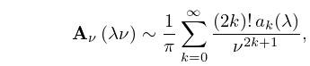
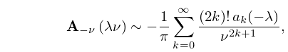
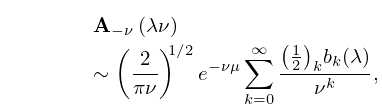
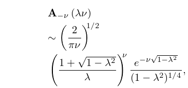
… ►Then …

6: 11.11 Asymptotic Expansions of Anger–Weber Functions

… ►

11.11.8 $${𝐀}_{\nu }\left(\lambda \nu \right)\sim \frac{1}{\pi }\sum _{k=0}^{\mathrm{\infty }}\frac{(2k)!a_k(\lambda )}{{\nu }^{2k+1}},$$ $\nu \to \mathrm{\infty }$, $|\mathrm{ph}\nu |\le \pi -\delta$,

ⓘ

Symbols:

${𝐀}_{\nu }\left(z\right)$: Anger–Weber function, $\sim$: Poincaré asymptotic expansion, $\pi$: the ratio of the circumference of a circle to its diameter, $!$: factorial (as in $n!$), $\mathrm{ph}$: phase, $\nu$: real or complex order, $k$: nonnegative integer, $\delta$: arbitrary small positive constant, $\lambda$: parameter and $a_k(\lambda )$: expansion function

Sources:

Meijer (1932); Watson (1944, §10.15); Olver (1997b, pp. 103 and 352); Nemes (2014b); Nemes (2014c)

Referenced by:

(11.11.18), (11.11.19), §11.11(iii)

Permalink:

http://dlmf.nist.gov/11.11.E8

Encodings:

pMML, png, TeX

Clarification (effective with 1.1.2):

The constraint which originally was $\nu \to \mathrm{\infty }$, , has been replaced to be $\nu \to \mathrm{\infty }$, $|\mathrm{ph}\nu |\le \pi -\delta$.

Suggested 2021-04-05 by Gergő Nemes

See also:

Annotations for §11.11(iii), §11.11 and Ch.11

… ►

11.11.10 $${𝐀}_{-\nu }\left(\lambda \nu \right)\sim -\frac{1}{\pi }\sum _{k=0}^{\mathrm{\infty }}\frac{(2k)!a_k(-\lambda )}{{\nu }^{2k+1}},$$ $\nu \to \mathrm{\infty }$, $|\mathrm{ph}\nu |\le \pi -\delta$.

ⓘ

Symbols:

${𝐀}_{\nu }\left(z\right)$: Anger–Weber function, $\sim$: Poincaré asymptotic expansion, $\pi$: the ratio of the circumference of a circle to its diameter, $!$: factorial (as in $n!$), $\mathrm{ph}$: phase, $\nu$: real or complex order, $k$: nonnegative integer, $\delta$: arbitrary small positive constant, $\lambda$: parameter and $a_k(\lambda )$: expansion function

Sources:

Meijer (1932); Watson (1944, §10.15); Olver (1997b, pp. 103 and 352); Nemes (2014b); Nemes (2014c)

Proof sketch:

Apply Laplace’s method to the integral (11.10.4).

Referenced by:

(11.11.18), (11.11.19), §11.11(iii), §11.11(iii)

Permalink:

http://dlmf.nist.gov/11.11.E10

Encodings:

pMML, png, TeX

Clarification (effective with 1.1.2):

The constraint which was originally $\nu \to +\mathrm{\infty }$, has been extended to be $\nu \to \mathrm{\infty }$, $|\mathrm{ph}\nu |\le \pi -\delta$.

Suggested 2021-04-05 by Gergő Nemes

See also:

Annotations for §11.11(iii), §11.11 and Ch.11

… ►

11.11.11 $${𝐀}_{-\nu }\left(\lambda \nu \right)\sim {\left(\frac{2}{\pi \nu }\right)}^{1/2}{\mathrm{e}}^{-\nu \mu }\sum _{k=0}^{\mathrm{\infty }}\frac{{\left(\frac{1}{2}\right)}_k{b}_k(\lambda )}{{\nu }^k},$$ $\nu \to \mathrm{\infty }$, $|\mathrm{ph}\nu |\le \frac{\pi }{2}-\delta$,

ⓘ

Symbols:

${\left(a\right)}_n$: Pochhammer’s symbol (or shifted factorial), ${𝐀}_{\nu }\left(z\right)$: Anger–Weber function, $\sim$: Poincaré asymptotic expansion, $\pi$: the ratio of the circumference of a circle to its diameter, $\mathrm{e}$: base of natural logarithm, $\mathrm{ph}$: phase, $\nu$: real or complex order, $k$: nonnegative integer, $\delta$: arbitrary small positive constant, $\lambda$: parameter and $b_k(\lambda )$: expansion function

Sources:

Dingle (1973, p. 388); Olver (1997b, pp. 103 and 352)

Proof sketch:

Derivable by applying Laplace’s method to the integral (11.10.4).

Permalink:

http://dlmf.nist.gov/11.11.E11

Encodings:

pMML, png, TeX

Clarification (effective with 1.1.2):

The constraint which was originally $\nu \to +\mathrm{\infty }$, has been extended to be $\nu \to \mathrm{\infty }$, $|\mathrm{ph}\nu |\le \frac{\pi }{2}-\delta$.

Suggested 2021-04-05 by Gergő Nemes

See also:

Annotations for §11.11(iii), §11.11 and Ch.11

… ►

11.11.14 $${𝐀}_{-\nu }\left(\lambda \nu \right)\sim \frac{1}{\pi \nu (\lambda -1)},$$ $\lambda >1$, $|\mathrm{ph}\nu |\le \pi -\delta$,

ⓘ

Symbols:

${𝐀}_{\nu }\left(z\right)$: Anger–Weber function, $\sim$: asymptotic equality, $\pi$: the ratio of the circumference of a circle to its diameter, $\mathrm{ph}$: phase, $\nu$: real or complex order, $\delta$: arbitrary small positive constant and $\lambda$: parameter

Source:

Olver (1997b, pp. 103 and 352)

Referenced by:

§11.11(iii)

Permalink:

http://dlmf.nist.gov/11.11.E14

Encodings:

pMML, png, TeX

Clarification (effective with 1.1.2):

The constraint has been extended to include $|\mathrm{ph}\nu |\le \pi -\delta$.

Suggested 2021-04-06 by Gergő Nemes

See also:

Annotations for §11.11(iii), §11.11 and Ch.11

►

11.11.15 $${𝐀}_{-\nu }\left(\lambda \nu \right)\sim {\left(\frac{2}{\pi \nu }\right)}^{1/2}{\left(\frac{1+\sqrt{1-{\lambda }^2}}{\lambda }\right)}^{\nu }\frac{{\mathrm{e}}^{-\nu \sqrt{1-{\lambda }^2}}}{{(1-{\lambda }^2)}^{1/4}},$$ , $|\mathrm{ph}\nu |\le \frac{\pi }{2}-\delta$.

ⓘ

Symbols:

${𝐀}_{\nu }\left(z\right)$: Anger–Weber function, $\sim$: asymptotic equality, $\pi$: the ratio of the circumference of a circle to its diameter, $\mathrm{e}$: base of natural logarithm, $\mathrm{ph}$: phase, $\nu$: real or complex order, $\delta$: arbitrary small positive constant and $\lambda$: parameter

Source:

Olver (1997b, pp. 103 and 352)

Permalink:

http://dlmf.nist.gov/11.11.E15

Encodings:

pMML, png, TeX

Clarification (effective with 1.1.2):

The constraint has been extended to include $|\mathrm{ph}\nu |\le \frac{\pi }{2}-\delta$.

Suggested 2021-04-06 by Gergő Nemes

See also:

Annotations for §11.11(iii), §11.11 and Ch.11

…

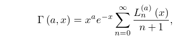
7: 8.7 Series Expansions

… ►

8.7.6 $$\mathrm{\Gamma }(a,x)=x^a{\mathrm{e}}^{-x}\sum _{n=0}^{\mathrm{\infty }}\frac{L_n^{(a)}\left(x\right)}{n+1},$$ $x>0$, .

ⓘ

Symbols:

$L_n^{(\alpha )}\left(x\right)$: Laguerre (or generalized Laguerre) polynomial, $\mathrm{e}$: base of natural logarithm, $\mathrm{\Gamma }(a,z)$: incomplete gamma function, $\mathrm{\Re }$: real part, $x$: real variable, $z$: complex variable, $a$: parameter and $n$: nonnegative integer

Proof sketch:

Integrate (18.12.13) from $z=0$ to $z=1$ and for the integral on the left-hand side use the substitution $z=\frac{t}{1+t}$. The resulting integral is (8.6.5). The constraint follows from (18.15.14).

Referenced by:

Erratum (V1.1.8) for Equation (8.7.6)

Permalink:

http://dlmf.nist.gov/8.7.E6

Encodings:

pMML, png, TeX

Addition (effective with 1.1.8):

The constraint was updated to include .

Suggested 2022-10-14 by Walter Gautschi

See also:

Annotations for §8.7 and Ch.8

…

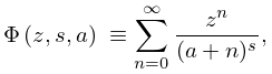
8: 25.14 Lerch’s Transcendent

… ►

25.14.1 $$\mathrm{\Phi }(z,s,a)\equiv \sum _{n=0}^{\mathrm{\infty }}\frac{z^n}{{(a+n)}^s},$$ ; $\mathrm{\Re }s>1,|z|=1$.

ⓘ

Defines:

$\mathrm{\Phi }(z,s,a)$: Lerch’s transcendent

Symbols:

$\equiv$: equals by definition, $\mathrm{\Re }$: real part, $n$: nonnegative integer, $a$: real or complex parameter, $s$: complex variable and $z$: complex variable

Keywords:

definition, infinite series, series representation

Source:

Erdélyi et al. (1953a, (1.11.1), p. 27)

Referenced by:

(25.14.2), (25.14.3), §25.14(ii), §25.14, Erratum (V1.0.21) for Equation (25.14.1)

Permalink:

http://dlmf.nist.gov/25.14.E1

Encodings:

pMML, png, TeX

Clarification (effective with 1.0.21):

The previous constraint $a\ne 0,-1,-2,\mathrm{\dots },$ was removed. A clarification regarding the correct constraints for Lerch’s transcendent $\mathrm{\Phi }(z,s,a)$ has been added in the text immediately below.

See also:

Annotations for §25.14(i), §25.14 and Ch.25

… ►

25.14.6 $$\mathrm{\Phi }(z,s,a)=\frac{1}{2}{a}^{-s}+{\int }_0^{\mathrm{\infty }}\frac{z^x}{{(a+x)}^s}dx-2{\int }_0^{\mathrm{\infty }}\frac{\sin \left(x\ln z-s\arctan \left(x/a\right)\right)}{{(a^2+x^2)}^{s/2}({\mathrm{e}}^{2\pi x}-1)}dx,$$ $\mathrm{\Re }a>0$ if ; $\mathrm{\Re }s>1$, $\mathrm{\Re }a>0$ if $\left|z\right|=1$.

ⓘ

Symbols:

$\mathrm{\Phi }(z,s,a)$: Lerch’s transcendent, $\pi$: the ratio of the circumference of a circle to its diameter, $dx$: differential of $x$ , $\mathrm{e}$: base of natural logarithm, $\int$: integral, $\arctan z$: arctangent function, $\ln z$: principal branch of logarithm function, $\mathrm{\Re }$: real part, $\sin z$: sine function, $x$: real variable, $a$: real or complex parameter, $s$: complex variable and $z$: complex variable

Keywords:

improper integral, integral representation

Source:

Erdélyi et al. (1953a, (1.11.4), p. 28)

Notes:

For the case see Erdélyi et al. (1953a, (1.11.4), p. 28). In the case $\left|z\right|=1$ one checks that the first integral converges absolutely iff $\mathrm{\Re }s>1$.

Referenced by:

Erratum (V1.1.4) for Equation (25.14.6)

Permalink:

http://dlmf.nist.gov/25.14.E6

Encodings:

pMML, png, TeX

Clarification (effective with 1.1.4):

The constraint which originally read “$\mathrm{\Re }s>0$ if ; $\mathrm{\Re }s>1$ if $|z|=1,\mathrm{\Re }a>0$” has been improved to be “$\mathrm{\Re }a>0$ if ; $\mathrm{\Re }s>1$, $\mathrm{\Re }a>0$ if $\left|z\right|=1$”.

Suggested 2021-08-23 by Gergő Nemes

See also:

Annotations for §25.14(ii), §25.14 and Ch.25

…

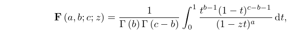
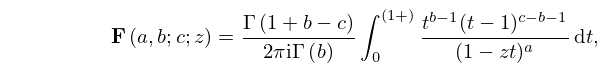
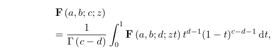
9: 15.6 Integral Representations

… ►

15.6.1 $$𝐅(a,b;c;z)=\frac{1}{\mathrm{\Gamma }\left(b\right)\mathrm{\Gamma }\left(c-b\right)}{\int }_0^1\frac{t^{b-1}{(1-t)}^{c-b-1}}{{(1-zt)}^a}dt,$$ ; $\mathrm{\Re }c>\mathrm{\Re }b>0$.

ⓘ

Symbols:

$\mathrm{\Gamma }\left(z\right)$: gamma function, $\pi$: the ratio of the circumference of a circle to its diameter, $dx$: differential of $x$ , $\int$: integral, $\mathrm{ph}$: phase, $\mathrm{\Re }$: real part, $𝐅(a,b;c;z)$ or $𝐅(\genfrac{}{}{0pt}{}{a,b}{c};z)$: $={}_2{}^{}𝐅_1^{}(a,b;c;z)$ Olver’s hypergeometric function, $z$: complex variable, $a$: real or complex parameter, $b$: real or complex parameter and $c$: real or complex parameter

Keywords:

Mellin transform

Referenced by:

§15.19(iii), (15.4.34), §15.6, §15.6, Erratum (V1.0.23) for Equations (15.6.1)–(15.6.9), Erratum (V1.0.23) for Equations (15.6.1)–(15.6.9)

Permalink:

http://dlmf.nist.gov/15.6.E1

Encodings:

pMML, png, TeX

Addition (effective with 1.0.23):

The Olver hypergeometric function $𝐅(a,b;c;z)$, previously omitted from the left-hand side to make the formula more concise, has been added. The constraint , originally mentioned in the text, has been directly added to the formula.

See also:

Annotations for §15.6 and Ch.15

►

15.6.2 $$𝐅(a,b;c;z)=\frac{\mathrm{\Gamma }\left(1+b-c\right)}{2\pi \mathrm{i}\mathrm{\Gamma }\left(b\right)}{\int }_0^{(1+)}\frac{t^{b-1}{(t-1)}^{c-b-1}}{{(1-zt)}^a}dt,$$ ; $c-b\ne 1,2,3,\mathrm{\dots }$, $\mathrm{\Re }b>0$.

ⓘ

Symbols:

$\mathrm{\Gamma }\left(z\right)$: gamma function, $\pi$: the ratio of the circumference of a circle to its diameter, $dx$: differential of $x$ , $\mathrm{i}$: imaginary unit, $\int$: integral, $\mathrm{ph}$: phase, $\mathrm{\Re }$: real part, $𝐅(a,b;c;z)$ or $𝐅(\genfrac{}{}{0pt}{}{a,b}{c};z)$: $={}_2{}^{}𝐅_1^{}(a,b;c;z)$ Olver’s hypergeometric function, $z$: complex variable, $a$: real or complex parameter, $b$: real or complex parameter and $c$: real or complex parameter

Keywords:

Mellin transform

Referenced by:

§15.6

Permalink:

http://dlmf.nist.gov/15.6.E2

Encodings:

pMML, png, TeX

Addition (effective with 1.0.23):

The Olver hypergeometric function $𝐅(a,b;c;z)$, previously omitted from the left-hand side to make the formula more concise, has been added. The constraint , originally mentioned in the text, has been directly added to the formula.

See also:

Annotations for §15.6 and Ch.15

… ►

15.6.6 $$𝐅(a,b;c;z)=\frac{1}{2\pi \mathrm{i}\mathrm{\Gamma }\left(a\right)\mathrm{\Gamma }\left(b\right)}{\int }_{-\mathrm{i}\mathrm{\infty }}^{\mathrm{i}\mathrm{\infty }}\frac{\mathrm{\Gamma }\left(a+t\right)\mathrm{\Gamma }\left(b+t\right)\mathrm{\Gamma }\left(-t\right)}{\mathrm{\Gamma }\left(c+t\right)}{(-z)}^{t}dt,$$ ; $a,b\ne 0,-1,-2,\mathrm{\dots }$.

ⓘ

Symbols:

$\mathrm{\Gamma }\left(z\right)$: gamma function, $\pi$: the ratio of the circumference of a circle to its diameter, $dx$: differential of $x$ , $\mathrm{i}$: imaginary unit, $\int$: integral, $\mathrm{ph}$: phase, $𝐅(a,b;c;z)$ or $𝐅(\genfrac{}{}{0pt}{}{a,b}{c};z)$: $={}_2{}^{}𝐅_1^{}(a,b;c;z)$ Olver’s hypergeometric function, $z$: complex variable, $a$: real or complex parameter, $b$: real or complex parameter and $c$: real or complex parameter

A&S Ref:

15.3.2 (modified)

Referenced by:

§15.6, §15.6, Erratum (V1.0.23) for Equations (15.6.1)–(15.6.9)

Permalink:

http://dlmf.nist.gov/15.6.E6

Encodings:

pMML, png, TeX

Addition (effective with 1.0.23):

The Olver hypergeometric function $𝐅(a,b;c;z)$, previously omitted from the left-hand side to make the formula more concise, has been added. The constraint , originally mentioned in the text, has been directly added to the formula.

See also:

Annotations for §15.6 and Ch.15

►

15.6.7 $$𝐅(a,b;c;z)=\frac{1}{2\pi \mathrm{i}\mathrm{\Gamma }\left(a\right)\mathrm{\Gamma }\left(b\right)\mathrm{\Gamma }\left(c-a\right)\mathrm{\Gamma }\left(c-b\right)}{\int }_{-\mathrm{i}\mathrm{\infty }}^{\mathrm{i}\mathrm{\infty }}\mathrm{\Gamma }\left(a+t\right)\mathrm{\Gamma }\left(b+t\right)\mathrm{\Gamma }\left(c-a-b-t\right)\mathrm{\Gamma }\left(-t\right){(1-z)}^{t}dt,$$ ; $a,b,c-a,c-b\ne 0,-1,-2,\mathrm{\dots }$.

ⓘ

Symbols:

$\mathrm{\Gamma }\left(z\right)$: gamma function, $\pi$: the ratio of the circumference of a circle to its diameter, $dx$: differential of $x$ , $\mathrm{i}$: imaginary unit, $\int$: integral, $\mathrm{ph}$: phase, $𝐅(a,b;c;z)$ or $𝐅(\genfrac{}{}{0pt}{}{a,b}{c};z)$: $={}_2{}^{}𝐅_1^{}(a,b;c;z)$ Olver’s hypergeometric function, $z$: complex variable, $a$: real or complex parameter, $b$: real or complex parameter and $c$: real or complex parameter

Referenced by:

§15.6, Erratum (V1.0.23) for Equations (15.6.1)–(15.6.9)

Permalink:

http://dlmf.nist.gov/15.6.E7

Encodings:

pMML, png, TeX

Addition (effective with 1.0.23):

The Olver hypergeometric function $𝐅(a,b;c;z)$, previously omitted from the left-hand side to make the formula more concise, has been added. The constraint , originally mentioned in the text, has been directly added to the formula.

See also:

Annotations for §15.6 and Ch.15

►

15.6.8 $$𝐅(a,b;c;z)=\frac{1}{\mathrm{\Gamma }\left(c-d\right)}{\int }_0^1𝐅(a,b;d;zt)t^{d-1}{(1-t)}^{c-d-1}dt,$$ ; $\mathrm{\Re }c>\mathrm{\Re }d>0$.

ⓘ

Symbols:

$\mathrm{\Gamma }\left(z\right)$: gamma function, $\pi$: the ratio of the circumference of a circle to its diameter, $dx$: differential of $x$ , $\int$: integral, $\mathrm{ph}$: phase, $\mathrm{\Re }$: real part, $𝐅(a,b;c;z)$ or $𝐅(\genfrac{}{}{0pt}{}{a,b}{c};z)$: $={}_2{}^{}𝐅_1^{}(a,b;c;z)$ Olver’s hypergeometric function, $z$: complex variable, $a$: real or complex parameter, $b$: real or complex parameter and $c$: real or complex parameter

Keywords:

Mellin transform

Proof sketch:

Follows from (15.6.9) with $\lambda =a+b$.

Referenced by:

(15.6.9), §15.6, §15.6, §15.6, §18.17(iv), Erratum (V1.0.14) for Equation (15.6.8), Erratum (V1.0.14) for Equation (15.6.8)

Permalink:

http://dlmf.nist.gov/15.6.E8

Encodings:

pMML, png, TeX

Addition (effective with 1.0.23):

The Olver hypergeometric function $𝐅(a,b;c;z)$, previously omitted from the left-hand side to make the formula more concise, has been added. The constraint , originally mentioned in the text, has been directly added to the formula.

See also:

Annotations for §15.6 and Ch.15

…

10: 33.14 Definitions and Basic Properties

… ►

33.14.13 $${\int }_0^{\mathrm{\infty }}s({ϵ}_1,\mathrm{\ell };r)s({ϵ}_2,\mathrm{\ell };r)dr=\delta \left({ϵ}_1-{ϵ}_2\right),$$ ${ϵ}_1,{ϵ}_2>0$,

ⓘ

Symbols:

$s(ϵ,\mathrm{\ell };r)$: regular Coulomb function, $\delta \left(x-a\right)$: Dirac delta (or Dirac delta function), $dx$: differential of $x$ , $\int$: integral, $\mathrm{\ell }$: nonnegative integer, $r$: real variable and $ϵ$: real parameter

Referenced by:

§13.10(vi), §13.23(v), §33.14(iv), Erratum (V1.0.24) for Subsection 33.14(iv)

Permalink:

http://dlmf.nist.gov/33.14.E13

Encodings:

pMML, png, TeX

Addition (effective with 1.0.24):

The constraint ${ϵ}_1,{ϵ}_2>0$ was added.

See also:

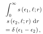
Annotations for §33.14(iv), §33.14 and Ch.33

…