over parametrized surface

♦ 1—10 of 149 matching pages ♦

(0.013 seconds)

1—10 of 149 matching pages

1: 21.7 Riemann Surfaces

§21.7 Riemann Surfaces

►

§21.7(i) Connection of Riemann Theta Functions to Riemann Surfaces

… ►For example, Figure 21.7.1 depicts a genus 2 surface. … ►

§21.7(iii) Frobenius’ Identity

… ►The genus of this surface is

g

. …

2: 1.6 Vectors and Vector-Valued Functions

… ►

§1.6(v) Surfaces and Integrals over Surfaces

►A parametrized surface

S

is defined by … ► ►The area

A(S)

of a parametrized smooth surface is given by … ►The integral of a continuous function

f(x,y,z)

over a surface

S

is …

3: 11.12 Physical Applications

§11.12 Physical Applications

►Applications of Struve functions occur in water-wave and surface-wave problems (Hirata (1975) and Ahmadi and Widnall (1985)), unsteady aerodynamics (Shaw (1985) and Wehausen and Laitone (1960)), distribution of fluid pressure over a vibrating disk (McLachlan (1934)), resistive MHD instability theory (Paris and Sy (1983)), and optical diffraction (Levine and Schwinger (1948)). …

4: 15.18 Physical Applications

… ►The hypergeometric function has allowed the development of “solvable” models for one-dimensional quantum scattering through and over barriers (Eckart (1930), Bhattacharjie and Sudarshan (1962)), and generalized to include position-dependent effective masses (Dekar et al. (1999)). ►More varied applications include photon scattering from atoms (Gavrila (1967)), energy distributions of particles in plasmas (Mace and Hellberg (1995)), conformal field theory of critical phenomena (Burkhardt and Xue (1991)), quantum chromo-dynamics (Atkinson and Johnson (1988)), and general parametrization of the effective potentials of interaction between atoms in diatomic molecules (Herrick and O’Connor (1998)).

5: Philip J. Davis

… ►In 1957, Davis took over as Chief, Numerical Analysis Section when John Todd and his wife Olga Taussky-Todd, feeling a strong pull toward teaching and research, left to pursue full-time positions at the California Institute of Technology. … ►NBS mathematician Irene Stegun took over management of the A&S project which was already well on its way, and led the work to publication in 1964. … ►Davis’s comments about our uninspired graphs sparked the research and design of techniques for creating interactive 3D visualizations of function surfaces, which grew in sophistication as our knowledge and the technology for developing 3D graphics on the web advanced over the years. …DLMF users can rotate, rescale, zoom and otherwise explore mathematical function surfaces. The surface color map can be changed from height-based to phase-based for complex valued functions, and density plots can be generated through strategic scaling. …

6: 21.10 Methods of Computation

… ►

§21.10(ii) Riemann Theta Functions Associated with a Riemann Surface

►In addition to evaluating the Fourier series, the main problem here is to compute a Riemann matrix originating from a Riemann surface. … ►

•

Belokolos et al. (1994, Chapter 5) and references therein. Here the Riemann surface is represented by the action of a Schottky group on a region of the complex plane. The same representation is used in Gianni et al. (1998).

►

•

Tretkoff and Tretkoff (1984). Here a Hurwitz system is chosen to represent the Riemann surface.

►

•

Deconinck and van Hoeij (2001). Here a plane algebraic curve representation of the Riemann surface is used.

7: About Color Map

… ►Surface visualizations in the DLMF represent functions of the form

z=f(x,y)

by the height

z

or the magnitude,

|z|

, for complex functions, over the

x\times y

plane. … ►To provide an easily interpreted encoding of surface heights, a rainbow-like mapping of height to color is used. … ►By painting the surfaces with a color that encodes the phase,

\operatorname{ph}f

, both the magnitude and phase of complex valued functions can be displayed. …

8: 21.1 Special Notation

… ► ►►►►

$g, h$	positive integers.
…
$a\circ b$	intersection index of $a$ and $b$ , two cycles lying on a closed surface. $a\circ b=0$ if $a$ and $b$ do not intersect. Otherwise $a\circ b$ gets an additive contribution from every intersection point. This contribution is $1$ if the basis of the tangent vectors of the $a$ and $b$ cycles (§21.7(i)) at the point of intersection is positively oriented; otherwise it is $-1$ .
$\oint_{a}\omega$	line integral of the differential $\omega$ over the cycle $a$ .

…

9: 14.30 Spherical and Spheroidal Harmonics

… ►

Y_{l}^{m}\left(\theta,\phi\right)

are known as surface harmonics of the first kind: tesseral for

|m|<l

and sectorial for

|m|=l

. … ►

14.30.11

\mathrm{L}^{2}Y_{{l},{m}}=\hbar^{2}l(l+1)Y_{{l},{m}},

l=0,1,2,\dots

ⓘ

Symbols:: $Y_{{\NVar{l}},{\NVar{m}}}\left(\NVar{\theta},\NVar{\phi}\right)$ : spherical harmonic, $m$ : integer, $l$ : nonnegative integer and $\mathrm{L}$ : angular momentum operator
Referenced by:: §18.39(ii)
Permalink:: http://dlmf.nist.gov/14.30.E11
Encodings:: pMML, png, TeX
See also:: Annotations for §14.30(iv), §14.30 and Ch.14

… ►

14.30.11_5

\mathrm{L}_{z}Y_{{l},{m}}=\hbar mY_{{l},{m}},

m=-l,-1+1,\dots,0,\dots,l-1,l

ⓘ

Symbols:: $Y_{{\NVar{l}},{\NVar{m}}}\left(\NVar{\theta},\NVar{\phi}\right)$ : spherical harmonic, $m$ : integer, $l$ : nonnegative integer and $\mathrm{L}_{z}$ : $z$ component of the angular momentum operator
Referenced by:: §14.30(iv), Erratum (V1.1.0) for Additions
Permalink:: http://dlmf.nist.gov/14.30.E11_5
Encodings:: pMML, png, TeX
Addition (effective with 1.1.0):: This equation was added.
See also:: Annotations for §14.30(iv), §14.30 and Ch.14

►where

\hbar

is the reduced Planck’s constant. … ►

14.30.13

\mathrm{L}_{z}=-\mathrm{i}\hbar\frac{\partial}{\partial\phi};

ⓘ

Defines:: $\mathrm{L}_{z}$ : $z$ component of the angular momentum operator (locally)
Symbols:: $\mathrm{i}$ : imaginary unit, $\frac{\partial\NVar{f}}{\partial\NVar{x}}$ : partial derivative of $f$ with respect to $x$ , $\,\partial\NVar{x}$ : partial differential of $x$ and $z$ : complex variable
Referenced by:: §14.30(iv), Erratum (V1.1.0) for Additions
Permalink:: http://dlmf.nist.gov/14.30.E13
Encodings:: pMML, png, TeX
Addition (effective with 1.1.0):: This equation was added.
See also:: Annotations for §14.30(iv), §14.30 and Ch.14

…

10: 21.4 Graphics

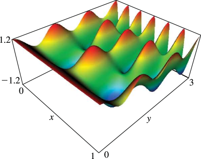
… ►Figure 21.4.1 provides surfaces of the scaled Riemann theta function

\hat{\theta}\left(\mathbf{z}\middle|\boldsymbol{{\Omega}}\right)

, with …This Riemann matrix originates from the Riemann surface represented by the algebraic curve

\mu^{3}-\lambda^{7}+2\lambda^{3}\mu=0

; compare §21.7(i). ►

…

Figure 21.4.1:

\hat{\theta}\left(\mathbf{z}\middle|\boldsymbol{{\Omega}}\right)

parametrized by (21.4.1). The surface plots are of

\hat{\theta}\left(x+iy,0\middle|\boldsymbol{{\Omega}}\right)

0\leq x\leq 1

0\leq y\leq 5

(suffix 1);

\hat{\theta}\left(x,y\middle|\boldsymbol{{\Omega}}\right)

0\leq x\leq 1

0\leq y\leq 1

(suffix 2);

\hat{\theta}\left(ix,iy\middle|\boldsymbol{{\Omega}}\right)

0\leq x\leq 5

0\leq y\leq 5

(suffix 3). …

… ►

See accompanying text — Figure 21.4.5: The real part of a genus 3 scaled Riemann theta function: $\Re\hat{\theta}\left(x+iy,0,0\middle|\boldsymbol{{\Omega}}_{2}\right)$ , $0\leq x\leq 1$ , $0\leq y\leq 3$ . This Riemann matrix originates from the genus 3 Riemann surface represented by the algebraic curve $\mu^{3}+2\mu-\lambda^{4}=0$ ; compare §21.7(i). Magnify 3D Help