open
(0.001 seconds)
11—20 of 195 matching pages
11: 28.17 Stability as
…
►If all solutions of (28.2.1) are bounded when along the real axis, then the corresponding pair of parameters is called stable.
…
►However, if , then always comprises an unstable pair.
…
►For real and
the stable regions are the open regions indicated in color in Figure 28.17.1.
…
12: 4.23 Inverse Trigonometric Functions
…
►The function assumes its principal value when ; elsewhere on the integration paths the branch is determined by continuity.
…
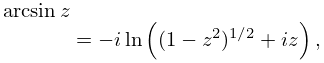
►
4.23.19
;
…
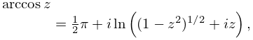
►
4.23.22
;
…
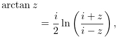
►
4.23.26
;
…
►where and in (4.23.34) and (4.23.35), and in (4.23.36).
…
13: 31.15 Stieltjes Polynomials
…
►then there are exactly
polynomials , each of which corresponds to each of the ways of distributing its zeros among intervals , .
…
►If the exponent and singularity parameters satisfy (31.15.5)–(31.15.6), then for every multi-index , where each is a nonnegative integer, there is a unique Stieltjes polynomial with zeros in the open interval for each .
…
►
31.15.8
,
►
31.15.9
,
…
►
31.15.10
…
14: 18.3 Definitions
…
►
Table 18.3.1: Orthogonality properties for classical OP’s: intervals, weight functions, standardizations, leading coefficients, and parameter constraints.
…
►
►
►
…
►For a finite system of Jacobi polynomials is orthogonal on with weight function .
For and a finite system of Jacobi polynomials (called pseudo Jacobi polynomials or Routh–Romanovski polynomials) is orthogonal on with .
…
| Name | Constraints | ||||||
|---|---|---|---|---|---|---|---|
| … | |||||||
| Chebyshev of second kind | |||||||
| Chebyshev of third kind | |||||||
| … | |||||||
15: 24.1 Special Notation
…
►
►
…
| integers, nonnegative unless stated otherwise. | |
| … | |
| greatest common divisor of . | |
| and relatively prime. | |
16: 23.20 Mathematical Applications
…
►Points on the curve can be parametrized by , , where and : in this case we write .
The curve is made into an abelian group (Macdonald (1968, Chapter 5)) by defining the zero element as the point at infinity, the negative of by , and generally on the curve iff the points , , are collinear.
…
►In terms of the addition law can be expressed , ; otherwise , where
…
►
always has the form (Mordell’s Theorem: Silverman and Tate (1992, Chapter 3, §5)); the determination of , the rank of , raises questions of great difficulty, many of which are still open.
…To determine , we make use of the fact that if then must be a divisor of ; hence there are only a finite number of possibilities for .
…
17: 18.31 Bernstein–Szegő Polynomials
…
►The Bernstein–Szegő polynomials
, , are orthogonal on with respect to three types of weight function: , , .
…
18: 7.24 Approximations
…
►
•
►
•
…
Schonfelder (1978) gives coefficients of Chebyshev expansions for on , for on , and for on (30D).
Shepherd and Laframboise (1981) gives coefficients of Chebyshev series for on (22D).
19: 23.1 Special Notation
…
►
►
…
| lattice in . | |
| … | |
| or | closed, or open, straight-line segment joining and , whether or not and are real. |
| … | |
| Cartesian product of groups and , that is, the set of all pairs of elements with group operation . | |
