on intervals

SearchAdvancedHelp

(0.003 seconds)

11—20 of 237 matching pages

11: 1.5 Calculus of Two or More Variables

… ►A function $f(x,y)$ is continuous at a point $(a,b)$ if … ► $f(x,y)$ has a local minimum (maximum) at $(a,b)$ if … ►for all $c_1\in [c_0,d)$ and all $x\in [a,b]$. … ►Let $f(x,y)$ be defined on a closed rectangle $R=[a,b]\times [c,d]$. … ►Moreover, if $a,b,c,d$ are finite or infinite constants and $f(x,y)$ is piecewise continuous on the set $(a,b)\times (c,d)$, then …

12: 4.3 Graphics

… ►

►►

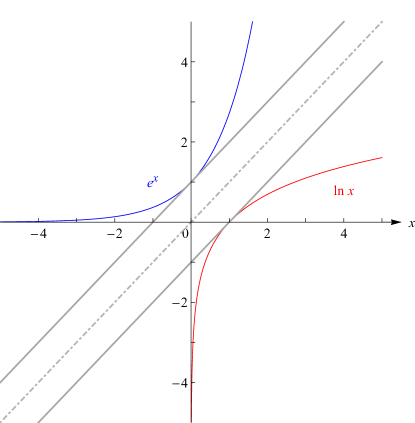
Figure 4.3.1: $\ln x$ and ${\mathrm{e}}^x$. Parallel tangent lines at $(1,0)$ and $(0,1)$ make evident the mirror symmetry across the line $y=x$, demonstrating the inverse relationship between the two functions. Magnify

… ►In the labeling of corresponding points $r$ is a real parameter that can lie anywhere in the interval $(0,\mathrm{\infty })$. …

13: 23.20 Mathematical Applications

… ►There is a unique point $z_0\in [{\omega }_1,{\omega }_1+{\omega }_3]\cup [{\omega }_1+{\omega }_3,{\omega }_3]$ such that $\mathrm{\wp }\left(z_0\right)=0$. … ►The two pairs of edges $[0,{\omega }_1]\cup [{\omega }_1,2{\omega }_3]$ and $[2{\omega }_3,2{\omega }_3-{\omega }_1]\cup [2{\omega }_3-{\omega }_1,0]$ of $R$ are each mapped strictly monotonically by $\mathrm{\wp }$ onto the real line, with $0\to \mathrm{\infty }$, ${\omega }_1\to e_1$, $2{\omega }_3\to -\mathrm{\infty }$; similarly for the other pair of edges. … ►The curve $C$ is made into an abelian group (Macdonald (1968, Chapter 5)) by defining the zero element $o=(0,1,0)$ as the point at infinity, the negative of $P=(x,y)$ by $-P=(x,-y)$, and generally $P_1+P_2+P_3=0$ on the curve iff the points $P_1$, $P_2$, $P_3$ are collinear. … ►In terms of $(x,y)$ the addition law can be expressed $(x,y)+o=(x,y)$, $(x,y)+(x,-y)=o$; otherwise $(x_1,y_1)+(x_2,y_2)=(x_3,y_3)$, where … ►To determine $T$, we make use of the fact that if $(x,y)\in T$ then $y^2$ must be a divisor of $\mathrm{\Delta }$; hence there are only a finite number of possibilities for $y$. …

14: Mathematical Introduction

… ► ►►►►

$ℂ$	complex plane (excluding infinity).
…
$(a,b)$	open interval in $ℝ$, or open straight-line segment joining $a$ and $b$ in $ℂ$.
$[a,b]$	closed interval in $ℝ$, or closed straight-line segment joining $a$ and $b$ in $ℂ$.

► ►►►

$(a,b]$ or $[a,b)$	half-closed intervals.
…
$[a_{j,k}]$ or $[a_{jk}]$	matrix with $(j,k)$th element $a_{j,k}$ or $a_{jk}$.
…

… ►This means that the variable $x$ ranges from 0 to 1 in intervals of 0. …

15: 4.23 Inverse Trigonometric Functions

… ►The function ${(1-t^2)}^{1/2}$ assumes its principal value when $t\in (-1,1)$; elsewhere on the integration paths the branch is determined by continuity. … ►

4.23.24 $$\arccos x=\mp \mathrm{i}\ln \left({(x^2-1)}^{1/2}+x\right),$$ $x\in [1,\mathrm{\infty })$,

ⓘ

Symbols:

$[a,b)$: half-closed interval, $\in$: element of, $\mathrm{i}$: imaginary unit, $\arccos z$: arccosine function, $\ln z$: principal branch of logarithm function and $x$: real variable

Permalink:

http://dlmf.nist.gov/4.23.E24

Encodings:

pMML, png, TeX

See also:

Annotations for §4.23(iv), §4.23(iv), §4.23 and Ch.4

►

4.23.25 $$\arccos x=\pi \mp \mathrm{i}\ln \left({(x^2-1)}^{1/2}-x\right),$$ $x\in (-\mathrm{\infty },-1]$,

ⓘ

Symbols:

$\pi$: the ratio of the circumference of a circle to its diameter, $\in$: element of, $\mathrm{i}$: imaginary unit, $\arccos z$: arccosine function, $\ln z$: principal branch of logarithm function, $(a,b]$: half-closed interval and $x$: real variable

Permalink:

http://dlmf.nist.gov/4.23.E25

Encodings:

pMML, png, TeX

See also:

Annotations for §4.23(iv), §4.23(iv), §4.23 and Ch.4

… ►

4.23.26 $$\arctan z=\frac{\mathrm{i}}{2}\ln \left(\frac{\mathrm{i}+z}{\mathrm{i}-z}\right),$$ $z/\mathrm{i}\in ℂ\setminus (-\mathrm{\infty },-1]\cup [1,\mathrm{\infty })$;

ⓘ

Symbols:

$[a,b)$: half-closed interval, $ℂ$: complex plane, $\in$: element of, $\mathrm{i}$: imaginary unit, $\arctan z$: arctangent function, $\ln z$: principal branch of logarithm function, $(a,b]$: half-closed interval, $\setminus$: set subtraction, $\cup$: union and $z$: complex variable

Referenced by:

§4.23(iv)

Permalink:

http://dlmf.nist.gov/4.23.E26

Encodings:

pMML, png, TeX

See also:

Annotations for §4.23(iv), §4.23(iv), §4.23 and Ch.4

… ►where $z=x+\mathrm{i}y$ and $\pm z\notin (1,\mathrm{\infty })$ in (4.23.34) and (4.23.35), and in (4.23.36). …

16: 29.9 Stability

… ►If $\nu$ is not an integer, then (29.2.1) is unstable iff $h\le a_{\nu }^0\left(k^2\right)$ or $h$ lies in one of the closed intervals with endpoints $a_{\nu }^m\left(k^2\right)$ and $b_{\nu }^m\left(k^2\right)$, $m=1,2,\mathrm{\dots }$. If $\nu$ is a nonnegative integer, then (29.2.1) is unstable iff $h\le a_{\nu }^0\left(k^2\right)$ or $h\in [b_{\nu }^m\left(k^2\right),a_{\nu }^m\left(k^2\right)]$ for some $m=1,2,\mathrm{\dots },\nu$.

17: 22.18 Mathematical Applications

… ►With $k\in [0,1]$ the mapping $z\to w=\mathrm{sn}(z,k)$ gives a conformal map of the closed rectangle $[-K,K]\times [0,K^{\prime }]$ onto the half-plane $\mathrm{\Im }w\ge 0$, with $0,\pm K,\pm K+\mathrm{i}{K}^{\prime },\mathrm{i}{K}^{\prime }$ mapping to $0,\pm 1,\pm k^{-2},\mathrm{\infty }$ respectively. The half-open rectangle $(-K,K)\times [-K^{\prime },K^{\prime }]$ maps onto $ℂ$ cut along the intervals $(-\mathrm{\infty },-1]$ and $[1,\mathrm{\infty })$. … ►For any two points $(x_1,y_1)$ and $(x_2,y_2)$ on this curve, their sum $(x_3,y_3)$, always a third point on the curve, is defined by the Jacobi–Abel addition law …

18: 8.1 Special Notation

… ►Alternative notations include: Prym’s functions $P_z(a)=\gamma (a,z)$, $Q_z(a)=\mathrm{\Gamma }(a,z)$, Nielsen (1906a, pp. 25–26), Batchelder (1967, p. 63); $(a,z)!=\gamma (a+1,z)$, $[a,z]!=\mathrm{\Gamma }(a+1,z)$, Dingle (1973); $B(a,b,x)={\mathrm{B}}_x(a,b)$, $I(a,b,x)=I_x(a,b)$, Magnus et al. (1966); $\mathrm{Si}(a,x)\to \mathrm{Si}(1-a,x)$, $\mathrm{Ci}(a,x)\to \mathrm{Ci}(1-a,x)$, Luke (1975).

19: 18.32 OP’s with Respect to Freud Weights

… ►All of these forms appear in applications, see §18.39(iii) and Table 18.39.1, albeit sometimes with $x\in [0,\mathrm{\infty })$, where the term half-Freud weight is used; or on $x\in [-1,1]$ or $[0,1]$, where the term Rys weight is employed, see Rys et al. (1983). For (generalized) Freud weights on a subinterval of $[0,\mathrm{\infty })$ see also Levin and Lubinsky (2005).

20: 18.24 Hahn Class: Asymptotic Approximations

… ►With $x=\lambda N$ and $\nu =n/N$, Li and Wong (2000) gives an asymptotic expansion for $K_n(x;p,N)$ as $n\to \mathrm{\infty }$, that holds uniformly for $\lambda$ and $\nu$ in compact subintervals of $(0,1)$. … ►With $\mu =N/n$ and $x$ fixed, Qiu and Wong (2004) gives an asymptotic expansion for $K_n(x;p,N)$ as $n\to \mathrm{\infty }$, that holds uniformly for $\mu \in [1,\mathrm{\infty })$. … ►Taken together, these expansions are uniformly valid for and for $a$ in unbounded intervals—each of which contains $[0,(1-\delta )n]$, where $\delta$ again denotes an arbitrary small positive constant. … ►This expansion is uniformly valid in any compact $x$-interval on the real line and is in terms of parabolic cylinder functions. … ►These approximations are in terms of Laguerre polynomials and hold uniformly for $\mathrm{ph}\left(x+i\lambda \right)\in [0,\pi ]$. …