on an interval

(0.004 seconds)

11—20 of 142 matching pages

11: 1.18 Linear Second Order Differential Operators and Eigenfunction Expansions

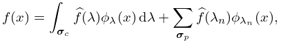
… ►Let

T

be a self-adjoint extension of differential operator

\mathcal{L}

of the form (1.18.28) and assume

T

has a complete set of

L^{2}

eigenfunctions,

\left\{\phi_{\lambda_{n}}(x)\right\}_{n=0}^{\infty}

x\in X=[a,b]

this latter being an appropriate sub-set of

\mathbb{R}

, or, in some cases

X=\mathbb{R}

itself, with real eigenvalues

\lambda_{n}

. … ►Let

T

be the self adjoint extension of a formally self-adjoint differential operator

\mathcal{L}

of the form (1.18.28) on an unbounded interval

X\subset\mathbb{R}

, which we will take as

X=[0,+\infty)

, and assume that

q(x)\to 0

monotonically as

x\to\infty

, and that the eigenfunctions are non-vanishing but bounded in this same limit. … ►

1.18.64

f(x)=\int_{\boldsymbol{\sigma}_{c}}\widehat{f}(\lambda)\phi_{\lambda}(x)\,% \mathrm{d}\lambda+\sum_{\boldsymbol{\sigma}_{p}}\widehat{f}(\lambda_{n})\phi_{% \lambda_{n}}(x),

f(x)\in C(X)\cap L^{2}\left(X\right)

ⓘ

Symbols:: $L^{2}\left(\NVar{X},\NVar{\,\mathrm{d}x}\right)$ : Lebesgue–Stieltjes measurable, square integrable, complex-valued functions, $\,\mathrm{d}\NVar{x}$ : differential of $x$ , $\in$ : element of, $\int$ : integral, $\cap$ : intersection, $C(\NVar{I})$ or $C(\NVar{a,b})$ : continuous on an interval $I$ or $(a,b)$ and $n$ : nonnegative integer
Permalink:: http://dlmf.nist.gov/1.18.E64
Encodings:: pMML, png, TeX
See also:: Annotations for §1.18(viii), §1.18 and Ch.1

… ►Thus, and this is a case where

q(x)

is not continuous, if

q(x)=-\alpha\delta\left(x-a\right)

\alpha>0

, there will be an

L^{2}

eigenfunction localized in the vicinity of

x=a

, with a negative eigenvalue, thus disjoint from the continuous spectrum on

[0,\infty)

. …

12: 18.33 Polynomials Orthogonal on the Unit Circle

… ►Let

\{p_{n}(x)\}

and

\{q_{n}(x)\}

n=0,1,\dots

, be OP’s with weight functions

w_{1}(x)

and

w_{2}(x)

, respectively, on

(-1,1)

. … ►After a quadratic transformation (18.2.23) this would express OP’s on

[-1,1]

with an even orthogonality measure in terms of the

\phi_{n}

. …

13: 15.19 Methods of Computation

… ►For

z\in\mathbb{R}

it is always possible to apply one of the linear transformations in §15.8(i) in such a way that the hypergeometric function is expressed in terms of hypergeometric functions with an argument in the interval

[0,\frac{1}{2}]

. …

14: 18.2 General Orthogonal Polynomials

… ►It is assumed throughout this chapter that for each polynomial

p_{n}(x)

that is orthogonal on an open interval

(a,b)

the variable

x

is confined to the closure of

(a,b)

unless indicated otherwise. (However, under appropriate conditions almost all equations given in the chapter can be continued analytically to various complex values of the variables.) … ►More generally than (18.2.1)–(18.2.3),

w(x)\,\mathrm{d}x

may be replaced in (18.2.1) by

\,\mathrm{d}\mu(x)

, where the measure

\mu

is the Lebesgue–Stieltjes measure

\mu_{\alpha}

corresponding to a bounded nondecreasing function

\alpha

on the closure of

(a,b)

with an infinite number of points of increase, and such that

\int_{a}^{b}|x|^{n}\,\mathrm{d}\mu(x)<\infty

for all

n

. … ►All

n

zeros of an OP

p_{n}(x)

are simple, and they are located in the interval of orthogonality

(a,b)

. … ►As a slight variant let

\{p_{n}(x)\}

be OP’s with respect to an even weight function

w(x)

(-1,1)

. … ►However, if OP’s have an orthogonality relation on a bounded interval, then their orthogonality measure is unique, up to a positive constant factor. …

15: 18.24 Hahn Class: Asymptotic Approximations

… ►With

x=\lambda N

and

\nu=n/N

, Li and Wong (2000) gives an asymptotic expansion for

K_{n}\left(x;p,N\right)

n\to\infty

, that holds uniformly for

\lambda

and

\nu

in compact subintervals of

(0,1)

. … ►With

\mu=N/n

and

x

fixed, Qiu and Wong (2004) gives an asymptotic expansion for

K_{n}\left(x;p,N\right)

n\to\infty

, that holds uniformly for

\mu\in[1,\infty)

. … ►Taken together, these expansions are uniformly valid for

-\infty<x<\infty

and for

a

in unbounded intervals—each of which contains

[0,(1-\delta)n]

, where

\delta

again denotes an arbitrary small positive constant. …

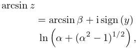
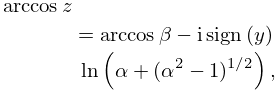
16: 4.23 Inverse Trigonometric Functions

… ►

4.23.34

\operatorname{arcsin}z=\operatorname{arcsin}\beta+\mathrm{i}\operatorname{sign% }\left(y\right)\ln\left(\alpha+(\alpha^{2}-1)^{1/2}\right),

ⓘ

Symbols:: $[\NVar{a},\NVar{b}]$ : closed interval, $\in$ : element of, $\mathrm{i}$ : imaginary unit, $\operatorname{arcsin}\NVar{z}$ : arcsine function, $\ln\NVar{z}$ : principal branch of logarithm function, $\notin$ : not an element of, $(\NVar{a},\NVar{b})$ : open interval, $\operatorname{sign}\NVar{x}$ : sign of, $x$ : real variable, $y$ : real variable, $z$ : complex variable, $\alpha$ and $\beta$
A&S Ref:: 4.4.37 (with the general value.)
Referenced by:: §4.23(vi), Erratum (V1.0.7) for Equations (4.23.34) and (4.23.35)
Permalink:: http://dlmf.nist.gov/4.23.E34
Encodings:: pMML, png, TeX
Errata (effective with 1.0.7):: Originally the factor $\operatorname{sign}\left(y\right)$ was missing from the second term on the right side of this equation. Also, the originally stated condition $x\in[-1,1]$ for this equation, stated on the line following (4.23.36), was replaced with the more general condition $\pm z\notin(1,\infty)$ .
Reported 2013-07-01 by Volker Thürey
See also:: Annotations for §4.23(vi), §4.23 and Ch.4

►

4.23.35

\operatorname{arccos}z=\operatorname{arccos}\beta-\mathrm{i}\operatorname{sign% }\left(y\right)\ln\left(\alpha+(\alpha^{2}-1)^{1/2}\right),

ⓘ

Symbols:: $[\NVar{a},\NVar{b}]$ : closed interval, $\in$ : element of, $\mathrm{i}$ : imaginary unit, $\operatorname{arccos}\NVar{z}$ : arccosine function, $\ln\NVar{z}$ : principal branch of logarithm function, $\notin$ : not an element of, $(\NVar{a},\NVar{b})$ : open interval, $\operatorname{sign}\NVar{x}$ : sign of, $x$ : real variable, $y$ : real variable, $z$ : complex variable, $\alpha$ and $\beta$
A&S Ref:: 4.4.38 (with the general value.)
Referenced by:: §4.23(vi), Erratum (V1.0.7) for Equations (4.23.34) and (4.23.35)
Permalink:: http://dlmf.nist.gov/4.23.E35
Encodings:: pMML, png, TeX
Errata (effective with 1.0.7):: Originally the factor $\operatorname{sign}\left(y\right)$ was missing from the second term on the right side of this equation. Also, the originally stated condition $x\in[-1,1]$ for this equation, stated on the line following (4.23.36), was replaced with the more general condition $\pm z\notin(1,\infty)$ .
Reported 2013-07-01 by Volker Thürey
See also:: Annotations for §4.23(vi), §4.23 and Ch.4

…

17: 18.36 Miscellaneous Polynomials

… ►These are OP’s on the interval

(-1,1)

with respect to an orthogonality measure obtained by adding constant multiples of “Dirac delta weights” at

-1

and

1

to the weight function for the Jacobi polynomials. …

18: 1.16 Distributions

… ►Let

\phi

be a function defined on an open interval

I=(a,b)

, which can be infinite. …

19: 1.5 Calculus of Two or More Variables

… ►If

F(x,y)

is continuously differentiable,

F(a,b)=0

, and

\ifrac{\partial F}{\partial y}\not=0

(a,b)

, then in a neighborhood of

(a,b)

, that is, an open disk centered at

a, b

, the equation

F(x,y)=0

defines a continuously differentiable function

y=g(x)

such that

F(x,g(x))=0

b=g(a)

, and

g^{\prime}(x)=-F_{x}/F_{y}

. …

20: 31.9 Orthogonality

… ►Here

\zeta

is an arbitrary point in the interval

(0,1)

. …