of the second kind

SearchAdvancedHelp

(0.003 seconds)

11—20 of 213 matching pages

11: 19.38 Approximations

… ►Minimax polynomial approximations (§3.11(i)) for $K\left(k\right)$ and $E\left(k\right)$ in terms of $m=k^2$ with can be found in Abramowitz and Stegun (1964, §17.3) with maximum absolute errors ranging from 4×10⁻⁵ to 2×10⁻⁸. Approximations of the same type for $K\left(k\right)$ and $E\left(k\right)$ for are given in Cody (1965a) with maximum absolute errors ranging from 4×10⁻⁵ to 4×10⁻¹⁸. …

12: 19.6 Special Cases

… ►

$E\left(1\right)=E^{\prime }\left(0\right)=1.$

… ►

§19.6(iii) $E(\varphi ,k)$

►

$E(0,k)=0,$

►

$E(\varphi ,0)=\varphi ,$

… ►

$E(\frac{1}{2}\pi ,k)=E\left(k\right).$

…

13: 26.21 Tables

§26.21 Tables

►Abramowitz and Stegun (1964, Chapter 24) tabulates binomial coefficients $\left(\genfrac{}{}{0.0pt}{}{m}{n}\right)$ for $m$ up to 50 and $n$ up to 25; extends Table 26.4.1 to $n=10$; tabulates Stirling numbers of the first and second kinds, $s(n,k)$ and $S(n,k)$, for $n$ up to 25 and $k$ up to $n$; tabulates partitions $p\left(n\right)$ and partitions into distinct parts $p(𝒟,n)$ for $n$ up to 500. … ►It also contains a table of Gaussian polynomials up to ${\left[\genfrac{}{}{0.0pt}{}{12}{6}\right]}_q$. …

14: 19.7 Connection Formulas

… ►

§19.7(i) Complete Integrals of the First and Second Kinds

… ►

19.7.1 $$E\left(k\right)K^{\prime }\left(k\right)+E^{\prime }\left(k\right)K\left(k\right)-K\left(k\right)K^{\prime }\left(k\right)=\frac{1}{2}\pi .$$

ⓘ

Symbols:

$\pi$: the ratio of the circumference of a circle to its diameter, $K^{\prime }\left(k\right)$: Legendre’s complementary complete elliptic integral of the first kind, $E^{\prime }\left(k\right)$: Legendre’s complementary complete elliptic integral of the second kind, $K\left(k\right)$: Legendre’s complete elliptic integral of the first kind, $E\left(k\right)$: Legendre’s complete elliptic integral of the second kind and $k$: real or complex modulus

Referenced by:

§19.21(i), §19.35(i), §19.7(i)

Permalink:

http://dlmf.nist.gov/19.7.E1

Encodings:

pMML, png, TeX

See also:

Annotations for §19.7(i), §19.7(i), §19.7 and Ch.19

… ►

$E\left(\mathrm{i}k/k^{\prime }\right)=(1/k^{\prime })E\left(k\right),$

►

$E\left(-\mathrm{i}{k}^{\prime }/k\right)=(1/k)E\left(k^{\prime }\right).$

… ►

$E(\varphi ,k_1)=(E(\beta ,k)-k_{}^{\prime }{}_{}{}^{2}F(\beta ,k))/k,$

…

15: 10.31 Power Series

… ►When $\nu$ is not an integer the corresponding expansion for $K_{\nu }\left(z\right)$ is obtained from (10.25.2) and (10.27.4). … ►

10.31.1 $$K_n\left(z\right)=\frac{1}{2}{(\frac{1}{2}z)}^{-n}\sum _{k=0}^{n-1}\frac{(n-k-1)!}{k!}{(-\frac{1}{4}{z}^2)}^k+{(-1)}^{n+1}\ln \left(\frac{1}{2}z\right)I_n\left(z\right)+{(-1)}^n\frac{1}{2}{(\frac{1}{2}z)}^n\sum _{k=0}^{\mathrm{\infty }}\left(\psi \left(k+1\right)+\psi \left(n+k+1\right)\right)\frac{{(\frac{1}{4}{z}^2)}^k}{k!(n+k)!},$$

ⓘ

Symbols:

$\psi \left(z\right)$: psi (or digamma) function, $!$: factorial (as in $n!$), $I_{\nu }\left(z\right)$: modified Bessel function of the first kind, $K_{\nu }\left(z\right)$: modified Bessel function of the second kind, $\ln z$: principal branch of logarithm function, $n$: integer, $k$: nonnegative integer and $z$: complex variable

A&S Ref:

9.6.11

Referenced by:

§10.30(i), §10.65(ii)

Permalink:

http://dlmf.nist.gov/10.31.E1

Encodings:

pMML, png, TeX

See also:

Annotations for §10.31 and Ch.10

… ►

10.31.2 $$K_0\left(z\right)=-\left(\ln \left(\frac{1}{2}z\right)+\gamma \right)I_0\left(z\right)+\frac{\frac{1}{4}{z}^2}{{(1!)}^2}+(1+\frac{1}{2})\frac{{(\frac{1}{4}{z}^2)}^2}{{(2!)}^2}+(1+\frac{1}{2}+\frac{1}{3})\frac{{(\frac{1}{4}{z}^2)}^3}{{(3!)}^2}+\mathrm{\cdots }.$$

ⓘ

Symbols:

$\gamma$: Euler’s constant, $!$: factorial (as in $n!$), $I_{\nu }\left(z\right)$: modified Bessel function of the first kind, $K_{\nu }\left(z\right)$: modified Bessel function of the second kind, $\ln z$: principal branch of logarithm function and $z$: complex variable

A&S Ref:

9.6.13

Referenced by:

§10.45

Permalink:

http://dlmf.nist.gov/10.31.E2

Encodings:

pMML, png, TeX

See also:

Annotations for §10.31 and Ch.10

…

16: 10.38 Derivatives with Respect to Order

… ►

10.38.2 $$\frac{\partial K_{\nu }\left(z\right)}{\partial \nu }=\frac{1}{2}\pi \csc \left(\nu \pi \right)\left(\frac{\partial I_{-\nu }\left(z\right)}{\partial \nu }-\frac{\partial I_{\nu }\left(z\right)}{\partial \nu }\right)-\pi \cot \left(\nu \pi \right)K_{\nu }\left(z\right),$$ $\nu \notin \mathbb{Z}$.

ⓘ

Symbols:

$\pi$: the ratio of the circumference of a circle to its diameter, $\csc z$: cosecant function, $\cot z$: cotangent function, $\mathbb{Z}$: set of all integers, $I_{\nu }\left(z\right)$: modified Bessel function of the first kind, $K_{\nu }\left(z\right)$: modified Bessel function of the second kind, $\notin$: not an element of, $\frac{\partial f}{\partial x}$: partial derivative of $f$ with respect to $x$ , $\partial x$: partial differential of $x$ , $z$: complex variable and $\nu$: complex parameter

A&S Ref:

9.6.43

Referenced by:

(10.38.1), §10.38, §10.38

Permalink:

http://dlmf.nist.gov/10.38.E2

Encodings:

pMML, png, TeX

See also:

Annotations for §10.38 and Ch.10

… ►

10.38.4 $${\frac{\partial K_{\nu }\left(z\right)}{\partial \nu }|}_{\nu =n}=\frac{n!}{2{(\frac{1}{2}z)}^n}\sum _{k=0}^{n-1}\frac{{(\frac{1}{2}z)}^k{K}_k\left(z\right)}{k!(n-k)}.$$

ⓘ

Symbols:

$!$: factorial (as in $n!$), $K_{\nu }\left(z\right)$: modified Bessel function of the second kind, $\frac{\partial f}{\partial x}$: partial derivative of $f$ with respect to $x$ , $\partial x$: partial differential of $x$ , $n$: integer, $k$: nonnegative integer, $z$: complex variable and $\nu$: complex parameter

A&S Ref:

9.6.45

Referenced by:

§10.38

Permalink:

http://dlmf.nist.gov/10.38.E4

Encodings:

pMML, png, TeX

See also:

Annotations for §10.38, §10.38 and Ch.10

►

${{\displaystyle \frac{\partial I_{\nu }\left(z\right)}{\partial \nu }}|}_{\nu =0}=-K_0\left(z\right),$

►

${{\displaystyle \frac{\partial K_{\nu }\left(z\right)}{\partial \nu }}|}_{\nu =0}=0.$

… ►

10.38.7 $${\frac{\partial K_{\nu }\left(x\right)}{\partial \nu }|}_{\nu =\pm \frac{1}{2}}=\pm \sqrt{\frac{\pi }{2x}}{E}_1\left(2x\right){\mathrm{e}}^x.$$

ⓘ

Symbols:

$\pi$: the ratio of the circumference of a circle to its diameter, $\mathrm{e}$: base of natural logarithm, $E_1\left(z\right)$: exponential integral, $K_{\nu }\left(z\right)$: modified Bessel function of the second kind, $\frac{\partial f}{\partial x}$: partial derivative of $f$ with respect to $x$ , $\partial x$: partial differential of $x$ , $x$: real variable and $\nu$: complex parameter

A&S Ref:

10.2.34 (corrected)

Referenced by:

§10.38, Ch.10

Permalink:

http://dlmf.nist.gov/10.38.E7

Encodings:

pMML, png, TeX

See also:

Annotations for §10.38, §10.38 and Ch.10

…

17: 10.27 Connection Formulas

… ►Other solutions of (10.25.1) are $I_{-\nu }\left(z\right)$ and $K_{-\nu }\left(z\right)$. … ►

10.27.2 $$I_{-\nu }\left(z\right)=I_{\nu }\left(z\right)+(2/\pi )\sin \left(\nu \pi \right)K_{\nu }\left(z\right),$$

ⓘ

Symbols:

$\pi$: the ratio of the circumference of a circle to its diameter, $I_{\nu }\left(z\right)$: modified Bessel function of the first kind, $K_{\nu }\left(z\right)$: modified Bessel function of the second kind, $\sin z$: sine function, $z$: complex variable and $\nu$: complex parameter

A&S Ref:

9.6.2

Permalink:

http://dlmf.nist.gov/10.27.E2

Encodings:

pMML, png, TeX

See also:

Annotations for §10.27 and Ch.10

►

10.27.3 $$K_{-\nu }\left(z\right)=K_{\nu }\left(z\right).$$

ⓘ

Symbols:

$K_{\nu }\left(z\right)$: modified Bessel function of the second kind, $z$: complex variable and $\nu$: complex parameter

A&S Ref:

9.6.6

Referenced by:

§10.25(iii), §10.30(i), §10.31, §10.47(ii)

Permalink:

http://dlmf.nist.gov/10.27.E3

Encodings:

pMML, png, TeX

See also:

Annotations for §10.27 and Ch.10

… ►

10.27.9 $$\pi \mathrm{i}{J}_{\nu }\left(z\right)={\mathrm{e}}^{-\nu \pi \mathrm{i}/2}{K}_{\nu }\left(z{\mathrm{e}}^{-\pi \mathrm{i}/2}\right)-{\mathrm{e}}^{\nu \pi \mathrm{i}/2}{K}_{\nu }\left(z{\mathrm{e}}^{\pi \mathrm{i}/2}\right),$$ $|\mathrm{ph}z|\le \frac{1}{2}\pi$.

ⓘ

Symbols:

$J_{\nu }\left(z\right)$: Bessel function of the first kind, $\pi$: the ratio of the circumference of a circle to its diameter, $\mathrm{e}$: base of natural logarithm, $\mathrm{i}$: imaginary unit, $K_{\nu }\left(z\right)$: modified Bessel function of the second kind, $\mathrm{ph}$: phase, $z$: complex variable and $\nu$: complex parameter

Referenced by:

§10.67(i)

Permalink:

http://dlmf.nist.gov/10.27.E9

Encodings:

pMML, png, TeX

See also:

Annotations for §10.27 and Ch.10

►

10.27.10 $$-\pi Y_{\nu }\left(z\right)={\mathrm{e}}^{-\nu \pi \mathrm{i}/2}{K}_{\nu }\left(z{\mathrm{e}}^{-\pi \mathrm{i}/2}\right)+{\mathrm{e}}^{\nu \pi \mathrm{i}/2}{K}_{\nu }\left(z{\mathrm{e}}^{\pi \mathrm{i}/2}\right),$$ $|\mathrm{ph}z|\le \frac{1}{2}\pi$.

ⓘ

Symbols:

$Y_{\nu }\left(z\right)$: Bessel function of the second kind, $\pi$: the ratio of the circumference of a circle to its diameter, $\mathrm{e}$: base of natural logarithm, $\mathrm{i}$: imaginary unit, $K_{\nu }\left(z\right)$: modified Bessel function of the second kind, $\mathrm{ph}$: phase, $z$: complex variable and $\nu$: complex parameter

Referenced by:

§10.43(iv)

Permalink:

http://dlmf.nist.gov/10.27.E10

Encodings:

pMML, png, TeX

See also:

Annotations for §10.27 and Ch.10

…

18: 19.3 Graphics

… ►

►►

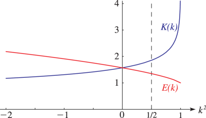
Figure 19.3.1: $K\left(k\right)$ and $E\left(k\right)$ as functions of $k^2$ for $-2\le k^2\le 1$. Graphs of $K^{\prime }\left(k\right)$ and $E^{\prime }\left(k\right)$ are the mirror images in the vertical line $k^2=\frac{1}{2}$. Magnify

… ►

►

►

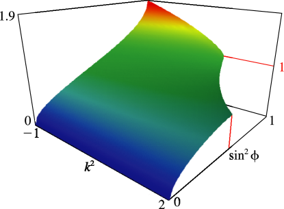
Figure 19.3.4: $E(\varphi ,k)$ as a function of $k^2$ and ${\sin }^2\varphi$ for $-1\le k^2\le 2$, $0\le {\sin }^2\varphi \le 1$. If ${\sin }^2\varphi =1$ ($\ge k^2$), then the function reduces to $E\left(k\right)$, with value 1 at $k^2=1$. … Magnify 3D Help

►

►

►

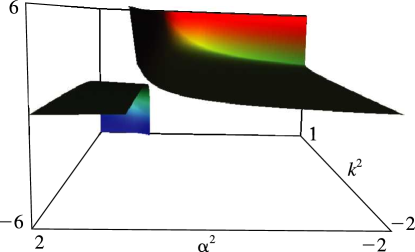
Figure 19.3.5: $\mathrm{\Pi }({\alpha }^2,k)$ as a function of $k^2$ and ${\alpha }^2$ for , $-2\le {\alpha }^2\le 2$. …As ${\alpha }^2\to 1+$ it has the limit $K\left(k\right)-(E\left(k\right)/k_{}^{\prime }{}_{}{}^2)$. … Magnify 3D Help

… ►

►

►

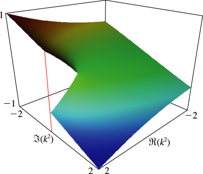
Figure 19.3.12: $\mathrm{\Im }\left(E\left(k\right)\right)$ as a function of complex $k^2$ for $-2\le \mathrm{\Re }\left(k^2\right)\le 2$, $-2\le \mathrm{\Im }\left(k^2\right)\le 2$. …On the upper edge of the branch cut ($k^2>1$) it has the (negative) value $K\left(k^{\prime }\right)-E\left(k^{\prime }\right)$, with limit 0 as $k^2\to 1+$. Magnify 3D Help

19: 19.39 Software

… ►Unless otherwise stated, the functions are $K\left(k\right)$ and $E\left(k\right)$, with $0\le k^2(=m)\le 1$. … ►Unless otherwise stated, the variables are real, and the functions are $F(\varphi ,k)$ and $E(\varphi ,k)$. ►For research software see Bulirsch (1965b, function $\mathrm{el2}$), Bulirsch (1969b, function $\mathrm{el3}$), Jefferson (1961), and Neuman (1969a, functions $E(\varphi ,k)$ and $\mathrm{\Pi }(\varphi ,k^2,k)$). …

20: 10.32 Integral Representations

… ►

10.32.5 $$K_0\left(z\right)=-\frac{1}{\pi }{\int }_0^{\pi }{\mathrm{e}}^{\pm z\cos \theta }\left(\gamma +\ln \left(2z{(\sin \theta )}^2\right)\right)d\theta .$$

ⓘ

Symbols:

$\gamma$: Euler’s constant, $\pi$: the ratio of the circumference of a circle to its diameter, $\cos z$: cosine function, $dx$: differential of $x$ , $\mathrm{e}$: base of natural logarithm, $\int$: integral, $K_{\nu }\left(z\right)$: modified Bessel function of the second kind, $\ln z$: principal branch of logarithm function, $\sin z$: sine function and $z$: complex variable

A&S Ref:

9.6.17

Permalink:

http://dlmf.nist.gov/10.32.E5

Encodings:

pMML, png, TeX

See also:

Annotations for §10.32(i), §10.32 and Ch.10

►

10.32.6 $$K_0\left(x\right)={\int }_0^{\mathrm{\infty }}\cos \left(x\sinh t\right)dt={\int }_0^{\mathrm{\infty }}\frac{\cos \left(xt\right)}{\sqrt{t^2+1}}dt,$$ $x>0$.

ⓘ

Symbols:

$\cos z$: cosine function, $dx$: differential of $x$ , $\sinh z$: hyperbolic sine function, $\int$: integral, $K_{\nu }\left(z\right)$: modified Bessel function of the second kind and $x$: real variable

A&S Ref:

9.6.21

Permalink:

http://dlmf.nist.gov/10.32.E6

Encodings:

pMML, png, TeX

See also:

Annotations for §10.32(i), §10.32 and Ch.10

… ►

10.32.17 $$K_{\mu }\left(z\right)K_{\nu }\left(z\right)=2{\int }_0^{\mathrm{\infty }}{K}_{\mu \pm \nu }\left(2z\cosh t\right)\cosh \left((\mu \mp \nu )t\right)dt,$$ .

ⓘ

Symbols:

$\pi$: the ratio of the circumference of a circle to its diameter, $dx$: differential of $x$ , $\cosh z$: hyperbolic cosine function, $\int$: integral, $K_{\nu }\left(z\right)$: modified Bessel function of the second kind, $\mathrm{ph}$: phase, $z$: complex variable and $\nu$: complex parameter

Permalink:

http://dlmf.nist.gov/10.32.E17

Encodings:

pMML, png, TeX

See also:

Annotations for §10.32(iii), §10.32 and Ch.10

►

10.32.18 $$K_{\nu }\left(z\right)K_{\nu }\left(\zeta \right)=\frac{1}{2}{\int }_0^{\mathrm{\infty }}\exp \left(-\frac{t}{2}-\frac{z^2+{\zeta }^2}{2t}\right)K_{\nu }\left(\frac{z\zeta }{t}\right)\frac{dt}{t},$$ , , .

ⓘ

Symbols:

$\pi$: the ratio of the circumference of a circle to its diameter, $dx$: differential of $x$ , $\exp z$: exponential function, $\int$: integral, $K_{\nu }\left(z\right)$: modified Bessel function of the second kind, $\mathrm{ph}$: phase, $z$: complex variable and $\nu$: complex parameter

Permalink:

http://dlmf.nist.gov/10.32.E18

Encodings:

pMML, png, TeX

See also:

Annotations for §10.32(iii), §10.32 and Ch.10

… ►For similar integrals for $J_{\nu }\left(z\right)K_{\nu }\left(z\right)$ and $I_{\nu }\left(z\right)K_{\nu }\left(z\right)$ see Paris and Kaminski (2001, p. 116). …