of the first kind

SearchAdvancedHelp

(0.011 seconds)

11—20 of 282 matching pages

11: 29.17 Other Solutions

… ►

29.17.1 $$F(z)=E(z){\int }_{\mathrm{i}{K}^{\prime }}^z\frac{du}{{(E(u))}^2}.$$

ⓘ

Symbols:

$K^{\prime }\left(k\right)$: Legendre’s complementary complete elliptic integral of the first kind, $dx$: differential of $x$ , $\mathrm{i}$: imaginary unit, $\int$: integral, $z$: complex variable and $k$: real parameter

Permalink:

http://dlmf.nist.gov/29.17.E1

Encodings:

pMML, png, TeX

See also:

Annotations for §29.17(i), §29.17 and Ch.29

… ►They are algebraic functions of $\mathrm{sn}(z,k)$, $\mathrm{cn}(z,k)$, and $\mathrm{dn}(z,k)$, and have primitive period $8K$. … ►Lamé–Wangerin functions are solutions of (29.2.1) with the property that ${(\mathrm{sn}(z,k))}^{1/2}w(z)$ is bounded on the line segment from $\mathrm{i}{K}^{\prime }$ to $2K+\mathrm{i}{K}^{\prime }$. …

12: 14.9 Connection Formulas

… ►

§14.9(i) Connections Between ${𝖯}_{\nu }^{\pm \mu }\left(x\right)$, ${𝖯}_{-\nu -1}^{\pm \mu }\left(x\right)$, ${𝖰}_{\nu }^{\pm \mu }\left(x\right)$, ${𝖰}_{-\nu -1}^{\mu }\left(x\right)$

… ►

${𝖯}_{-\nu -1}^{\mu }\left(x\right)={𝖯}_{\nu }^{\mu }\left(x\right),$

►

${𝖯}_{-\nu -1}^{-\mu }\left(x\right)={𝖯}_{\nu }^{-\mu }\left(x\right),$

… ►

§14.9(ii) Connections Between ${𝖯}_{\nu }^{\pm \mu }\left(\pm x\right)$, ${𝖰}_{\nu }^{-\mu }\left(\pm x\right)$, ${𝖰}_{\nu }^{\mu }\left(x\right)$

… ►

$P_{-\nu -1}^{\mu }\left(x\right)=P_{\nu }^{\mu }\left(x\right),$

…

13: 14.33 Tables

… ►

Abramowitz and Stegun (1964, Chapter 8) tabulates ${𝖯}_n\left(x\right)$ for $n=0(1)3,9,10$, $x=0(.01)1$, 5–8D; ${𝖯}_n^{\prime }\left(x\right)$ for $n=1(1)4,9,10$, $x=0(.01)1$, 5–7D; ${𝖰}_n\left(x\right)$ and ${𝖰}_n^{\prime }\left(x\right)$ for $n=0(1)3,9,10$, $x=0(.01)1$, 6–8D; $P_n\left(x\right)$ and $P_n^{\prime }\left(x\right)$ for $n=0(1)5,9,10$, $x=1(.2)10$, 6S; $Q_n\left(x\right)$ and $Q_n^{\prime }\left(x\right)$ for $n=0(1)3,9,10$, $x=1(.2)10$, 6S. (Here primes denote derivatives with respect to $x$.)

►

Zhang and Jin (1996, Chapter 4) tabulates ${𝖯}_n\left(x\right)$ for $n=2(1)5,10$, $x=0(.1)1$, 7D; ${𝖯}_n\left(\cos \theta \right)$ for $n=1(1)4,10$, $\theta =0(5^{\circ }){90}^{\circ }$, 8D; ${𝖰}_n\left(x\right)$ for $n=0(1)2,10$, $x=0(.1)0.9$, 8S; ${𝖰}_n\left(\cos \theta \right)$ for $n=0(1)3,10$, $\theta =0(5^{\circ }){90}^{\circ }$, 8D; ${𝖯}_n^m\left(x\right)$ for $m=1(1)4$, $n-m=0(1)2$, $n=10$, $x=0,0.5$, 8S; ${𝖰}_n^m\left(x\right)$ for $m=1(1)4$, $n=0(1)2,10$, 8S; ${𝖯}_{\nu }^m\left(\cos \theta \right)$ for $m=0(1)3$, $\nu =0(.25)5$, $\theta =0({15}^{\circ }){90}^{\circ }$, 5D; $P_n\left(x\right)$ for $n=2(1)5,10$, $x=1(1)10$, 7S; $Q_n\left(x\right)$ for $n=0(1)2,10$, $x=2(1)10$, 8S. Corresponding values of the derivative of each function are also included, as are 6D values of the first 5 $\nu$-zeros of ${𝖯}_{\nu }^m\left(\cos \theta \right)$ and of its derivative for $m=0(1)4$, $\theta ={10}^{\circ },{30}^{\circ },{150}^{\circ }$.

►

Belousov (1962) tabulates ${𝖯}_n^m\left(\cos \theta \right)$ (normalized) for $m=0(1)36$, $n-m=0(1)56$, $\theta =0({2.5}^{\circ }){90}^{\circ }$, 6D.

►

Žurina and Karmazina (1964, 1965) tabulate the conical functions ${𝖯}_{-\frac{1}{2}+\mathrm{i}\tau }\left(x\right)$ for $\tau =0(.01)50$, $x=-0.9(.1)0.9$, 7S; $P_{-\frac{1}{2}+\mathrm{i}\tau }\left(x\right)$ for $\tau =0(.01)50$, $x=1.1(.1)2(.2)5(.5)10(10)60$, 7D. Auxiliary tables are included to facilitate computation for larger values of $\tau$ when .

►

Žurina and Karmazina (1963) tabulates the conical functions ${𝖯}_{-\frac{1}{2}+\mathrm{i}\tau }^1\left(x\right)$ for $\tau =0(.01)25$, $x=-0.9(.1)0.9$, 7S; $P_{-\frac{1}{2}+\mathrm{i}\tau }^1\left(x\right)$ for $\tau =0(.01)25$, $x=1.1(.1)2(.2)5(.5)10(10)60$, 7S. Auxiliary tables are included to assist computation for larger values of $\tau$ when .

…

14: 14.18 Sums

… ►

14.18.1 $${𝖯}_{\nu }\left(\cos {\theta }_1\cos {\theta }_2+\sin {\theta }_1\sin {\theta }_2\cos \varphi \right)={𝖯}_{\nu }\left(\cos {\theta }_1\right){𝖯}_{\nu }\left(\cos {\theta }_2\right)+2\sum _{m=1}^{\mathrm{\infty }}{(-1)}^m{𝖯}_{\nu }^{-m}\left(\cos {\theta }_1\right){𝖯}_{\nu }^m\left(\cos {\theta }_2\right)\cos \left(m\varphi \right),$$

ⓘ

Symbols:

: Ferrers function of the first kind, $\cos z$: cosine function, ${𝖯}_{\nu }\left(x\right)={𝖯}_{\nu }^0\left(x\right)$: Ferrers function of the first kind, $\sin z$: sine function, $m$: nonnegative integer, $\nu$: general degree, ${\theta }_1$, ${\theta }_2$: real and $\varphi$: real

Referenced by:

§14.18(ii), §14.18(ii)

Permalink:

http://dlmf.nist.gov/14.18.E1

Encodings:

pMML, png, TeX

See also:

Annotations for §14.18(ii), §14.18 and Ch.14

►

14.18.2 $${𝖯}_n\left(\cos {\theta }_1\cos {\theta }_2+\sin {\theta }_1\sin {\theta }_2\cos \varphi \right)=\sum _{m=-n}^n{(-1)}^m{𝖯}_n^{-m}\left(\cos {\theta }_1\right){𝖯}_n^m\left(\cos {\theta }_2\right)\cos \left(m\varphi \right).$$

ⓘ

Symbols:

: Ferrers function of the first kind, $\cos z$: cosine function, ${𝖯}_{\nu }\left(x\right)={𝖯}_{\nu }^0\left(x\right)$: Ferrers function of the first kind, $\sin z$: sine function, $m$: nonnegative integer, $n$: nonnegative integer, ${\theta }_1$, ${\theta }_2$: real and $\varphi$: real

Referenced by:

§14.18(ii), §14.18(ii)

Permalink:

http://dlmf.nist.gov/14.18.E2

Encodings:

pMML, png, TeX

See also:

Annotations for §14.18(ii), §14.18 and Ch.14

… ►

14.18.3 $${𝖰}_{\nu }\left(\cos {\theta }_1\cos {\theta }_2+\sin {\theta }_1\sin {\theta }_2\cos \varphi \right)={𝖯}_{\nu }\left(\cos {\theta }_1\right){𝖰}_{\nu }\left(\cos {\theta }_2\right)+2\sum _{m=1}^{\mathrm{\infty }}{(-1)}^m{𝖯}_{\nu }^{-m}\left(\cos {\theta }_1\right){𝖰}_{\nu }^m\left(\cos {\theta }_2\right)\cos \left(m\varphi \right).$$

ⓘ

Symbols:

: Ferrers function of the first kind, : Ferrers function of the second kind, $\cos z$: cosine function, ${𝖯}_{\nu }\left(x\right)={𝖯}_{\nu }^0\left(x\right)$: Ferrers function of the first kind, ${𝖰}_{\nu }\left(x\right)={𝖰}_{\nu }^0\left(x\right)$: Ferrers function of the second kind, $\sin z$: sine function, $m$: nonnegative integer, $\nu$: general degree, ${\theta }_1$, ${\theta }_2$: real and $\varphi$: real

Referenced by:

§14.18(ii), Ch.14

Permalink:

http://dlmf.nist.gov/14.18.E3

Encodings:

pMML, png, TeX

See also:

Annotations for §14.18(ii), §14.18 and Ch.14

… ►

14.18.6 $$(x-y)\sum _{k=0}^n(2k+1)P_k\left(x\right)P_k\left(y\right)=(n+1)\left(P_{n+1}\left(x\right)P_n\left(y\right)-P_n\left(x\right)P_{n+1}\left(y\right)\right),$$

ⓘ

Symbols:

$P_{\nu }\left(z\right)=P_{\nu }^0\left(z\right)$: Legendre function of the first kind and $n$: nonnegative integer

A&S Ref:

8.9.1

Referenced by:

Erratum (V1.0.7) for Subsection 14.18(iii)

Permalink:

http://dlmf.nist.gov/14.18.E6

Encodings:

pMML, png, TeX

See also:

Annotations for §14.18(iii), §14.18(iii), §14.18 and Ch.14

►

14.18.7 $$(x-y)\sum _{k=0}^n(2k+1)P_k\left(x\right)Q_k\left(y\right)=(n+1)\left(P_{n+1}\left(x\right)Q_n\left(y\right)-P_n\left(x\right)Q_{n+1}\left(y\right)\right)-1.$$

ⓘ

Symbols:

$P_{\nu }\left(z\right)=P_{\nu }^0\left(z\right)$: Legendre function of the first kind, $Q_{\nu }\left(z\right)=Q_{\nu }^0\left(z\right)$: Legendre function of the second kind and $n$: nonnegative integer

A&S Ref:

8.9.2

Referenced by:

§14.18(iii), Erratum (V1.0.7) for Subsection 14.18(iii)

Permalink:

http://dlmf.nist.gov/14.18.E7

Encodings:

pMML, png, TeX

See also:

Annotations for §14.18(iii), §14.18(iii), §14.18 and Ch.14

…

15: 14.4 Graphics

… ►

►►

Figure 14.4.1: ${𝖯}_{\nu }^0\left(x\right)$, $\nu =0,\frac{1}{2},1,2,4$. Magnify

►

►►

Figure 14.4.2: ${𝖰}_{\nu }^0\left(x\right)$, $\nu =0,\frac{1}{2},1,2,4$. Magnify

►

►►

Figure 14.4.3: ${𝖯}_{\nu }^{-1/2}\left(x\right)$, $\nu =0,\frac{1}{2},1,2,4$. Magnify

►

►►

Figure 14.4.4: ${𝖰}_{\nu }^{1/2}\left(x\right)$, $\nu =0,\frac{1}{2},1,2,4$. Magnify

►

►►

Figure 14.4.5: ${𝖯}_{\nu }^{-1}\left(x\right)$, $\nu =0,\frac{1}{2},1,2,4$. Magnify

…

16: 29.4 Graphics

… ►

►►

Figure 29.4.13: ${\mathrm{𝐸𝑐}}_{1.5}^m(x,0.5)$ for $-2K\le x\le 2K$, $m=0,1,2$. $K=1.85407\mathrm{\dots }$. Magnify

►

►►

Figure 29.4.14: ${\mathrm{𝐸𝑠}}_{1.5}^m(x,0.5)$ for $-2K\le x\le 2K$, $m=1,2,3$. $K=1.85407\mathrm{\dots }$. Magnify

►

►►

Figure 29.4.15: ${\mathrm{𝐸𝑐}}_{1.5}^m(x,0.1)$ for $-2K\le x\le 2K$, $m=0,1,2$. $K=1.61244\mathrm{\dots }$. Magnify

►

►►

Figure 29.4.16: ${\mathrm{𝐸𝑠}}_{1.5}^m(x,0.1)$ for $-2K\le x\le 2K$, $m=1,2,3$. $K=1.61244\mathrm{\dots }$. Magnify

►

►►

Figure 29.4.17: ${\mathrm{𝐸𝑐}}_{1.5}^m(x,0.9)$ for $-2K\le x\le 2K$, $m=0,1,2$. $K=2.57809\mathrm{\dots }$. Magnify

…

17: 10.26 Graphics

… ►

►►

Figure 10.26.1: $I_0\left(x\right)$, $I_1\left(x\right)$, $K_0\left(x\right)$, $K_1\left(x\right)$, $0\le x\le 3$. Magnify

►

►►

Figure 10.26.2: ${\mathrm{e}}^{-x}{I}_0\left(x\right)$, ${\mathrm{e}}^{-x}{I}_1\left(x\right)$, ${\mathrm{e}}^x{K}_0\left(x\right)$, ${\mathrm{e}}^x{K}_1\left(x\right)$, $0\le x\le 10$. Magnify

… ►

►►

Figure 10.26.7: ${\tilde{I}}_{1/2}\left(x\right)$, ${\tilde{K}}_{1/2}\left(x\right)$, $0.01\le x\le 3$. Magnify

►

►►

Figure 10.26.8: ${\tilde{I}}_1\left(x\right)$, ${\tilde{K}}_1\left(x\right)$, $0.01\le x\le 3$. Magnify

►

►►

Figure 10.26.9: ${\tilde{I}}_5\left(x\right)$, ${\tilde{K}}_5\left(x\right)$, $0.01\le x\le 3$. Magnify

…

18: 14.11 Derivatives with Respect to Degree or Order

… ►

14.11.1 $$\frac{\partial }{\partial \nu }{𝖯}_{\nu }^{\mu }\left(x\right)=\pi \cot \left(\nu \pi \right){𝖯}_{\nu }^{\mu }\left(x\right)-\frac{1}{\pi }{𝖠}_{\nu }^{\mu }(x),$$

ⓘ

Symbols:

: Ferrers function of the first kind, $\pi$: the ratio of the circumference of a circle to its diameter, $\cot z$: cotangent function, $\frac{\partial f}{\partial x}$: partial derivative of $f$ with respect to $x$ , $\partial x$: partial differential of $x$ , $x$: real variable, $\mu$: general order, $\nu$: general degree and ${𝖠}_{\nu }^{\mu }(x)$

Referenced by:

§14.11, §14.11

Permalink:

http://dlmf.nist.gov/14.11.E1

Encodings:

pMML, png, TeX

See also:

Annotations for §14.11 and Ch.14

… ►

14.11.4 $${\frac{\partial }{\partial \mu }{𝖯}_{\nu }^{\mu }\left(x\right)|}_{\mu =0}=\left(\psi \left(-\nu \right)-\pi \cot \left(\nu \pi \right)\right){𝖯}_{\nu }\left(x\right)+{𝖰}_{\nu }\left(x\right),$$

ⓘ

Symbols:

: Ferrers function of the first kind, $\pi$: the ratio of the circumference of a circle to its diameter, $\cot z$: cotangent function, $\psi \left(z\right)$: psi (or digamma) function, $\frac{\partial f}{\partial x}$: partial derivative of $f$ with respect to $x$ , $\partial x$: partial differential of $x$ , ${𝖯}_{\nu }\left(x\right)={𝖯}_{\nu }^0\left(x\right)$: Ferrers function of the first kind, ${𝖰}_{\nu }\left(x\right)={𝖰}_{\nu }^0\left(x\right)$: Ferrers function of the second kind, $x$: real variable, $\mu$: general order and $\nu$: general degree

Referenced by:

§14.11, §14.11

Permalink:

http://dlmf.nist.gov/14.11.E4

Encodings:

pMML, png, TeX

See also:

Annotations for §14.11 and Ch.14

►

14.11.5 $${\frac{\partial }{\partial \mu }{𝖰}_{\nu }^{\mu }\left(x\right)|}_{\mu =0}=-\frac{1}{4}{\pi }^2{𝖯}_{\nu }\left(x\right)+\left(\psi \left(-\nu \right)-\pi \cot \left(\nu \pi \right)\right){𝖰}_{\nu }\left(x\right).$$

ⓘ

Symbols:

: Ferrers function of the second kind, $\pi$: the ratio of the circumference of a circle to its diameter, $\cot z$: cotangent function, $\psi \left(z\right)$: psi (or digamma) function, $\frac{\partial f}{\partial x}$: partial derivative of $f$ with respect to $x$ , $\partial x$: partial differential of $x$ , ${𝖯}_{\nu }\left(x\right)={𝖯}_{\nu }^0\left(x\right)$: Ferrers function of the first kind, ${𝖰}_{\nu }\left(x\right)={𝖰}_{\nu }^0\left(x\right)$: Ferrers function of the second kind, $x$: real variable, $\mu$: general order and $\nu$: general degree

Referenced by:

§14.11

Permalink:

http://dlmf.nist.gov/14.11.E5

Encodings:

pMML, png, TeX

See also:

Annotations for §14.11 and Ch.14

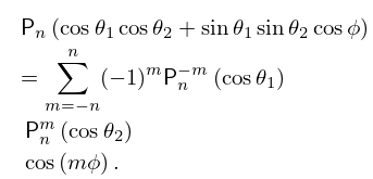
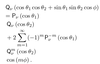
►(14.11.1) holds if ${𝖯}_{\nu }^{\mu }\left(x\right)$ is replaced by $P_{\nu }^{\mu }\left(x\right)$, provided that the factor ${((1+x)/(1-x))}^{\mu /2}$ in (14.11.3) is replaced by ${((x+1)/(x-1))}^{\mu /2}$. (14.11.4) holds if ${𝖯}_{\nu }^{\mu }\left(x\right)$, ${𝖯}_{\nu }\left(x\right)$, and ${𝖰}_{\nu }\left(x\right)$ are replaced by $P_{\nu }^{\mu }\left(x\right)$, $P_{\nu }\left(x\right)$, and $Q_{\nu }\left(x\right)$, respectively. …

19: 14.17 Integrals

… ►

14.17.3 $$\int x{𝖯}_{\nu }^{\mu }\left(x\right){𝖰}_{\nu }^{\mu }\left(x\right)dx=\frac{1}{2\nu (\nu +1)}\left(({\mu }^2-(\nu +1)(\nu +x^2)){𝖯}_{\nu }^{\mu }\left(x\right){𝖰}_{\nu }^{\mu }\left(x\right)+(\nu +1)(\nu -\mu +1)x({𝖯}_{\nu }^{\mu }\left(x\right){𝖰}_{\nu +1}^{\mu }\left(x\right)+{𝖯}_{\nu +1}^{\mu }\left(x\right){𝖰}_{\nu }^{\mu }\left(x\right))-{(\nu -\mu +1)}^2{𝖯}_{\nu +1}^{\mu }\left(x\right){𝖰}_{\nu +1}^{\mu }\left(x\right)\right),$$ $\nu \ne 0,-1$.

ⓘ

Symbols:

: Ferrers function of the first kind, : Ferrers function of the second kind, $dx$: differential of $x$ , $\int$: integral, $x$: real variable, $\mu$: general order and $\nu$: general degree

Referenced by:

§14.17(i)

Permalink:

http://dlmf.nist.gov/14.17.E3

Encodings:

pMML, png, TeX

See also:

Annotations for §14.17(i), §14.17 and Ch.14

►

14.17.4 $$\int \frac{x}{{\left(1-x^2\right)}^{3/2}}{𝖯}_{\nu }^{\mu }\left(x\right){𝖰}_{\nu }^{\mu }\left(x\right)dx=\frac{1}{\left(1-4{\mu }^2\right){\left(1-x^2\right)}^{1/2}}\left((1-2{\mu }^2+2\nu (\nu +1)){𝖯}_{\nu }^{\mu }\left(x\right){𝖰}_{\nu }^{\mu }\left(x\right)+(2\nu +1)(\mu -\nu -1)x({𝖯}_{\nu }^{\mu }\left(x\right){𝖰}_{\nu +1}^{\mu }\left(x\right)+{𝖯}_{\nu +1}^{\mu }\left(x\right){𝖰}_{\nu }^{\mu }\left(x\right))+2{(\mu -\nu -1)}^2{𝖯}_{\nu +1}^{\mu }\left(x\right){𝖰}_{\nu +1}^{\mu }\left(x\right)\right),$$ $\mu \ne \pm \frac{1}{2}$.

ⓘ

Symbols:

: Ferrers function of the first kind, : Ferrers function of the second kind, $dx$: differential of $x$ , $\int$: integral, $x$: real variable, $\mu$: general order and $\nu$: general degree

Referenced by:

§14.17(i)

Permalink:

http://dlmf.nist.gov/14.17.E4

Encodings:

pMML, png, TeX

See also:

Annotations for §14.17(i), §14.17 and Ch.14

►In (14.17.1)–(14.17.4), $𝖯$ may be replaced by $𝖰$, and in (14.17.3) and (14.17.4), $𝖰$ may be replaced by $𝖯$. … ►

14.17.15 $${\int }_{-1}^1{𝖯}_{\nu }\left(x\right){𝖰}_{\nu }\left(x\right)dx=-\frac{\sin \left(2\nu \pi \right){\psi }^{\prime }\left(\nu +1\right)}{\pi (2\nu +1)},$$ $\mathrm{\Re }\nu >0$.

ⓘ

Symbols:

$\pi$: the ratio of the circumference of a circle to its diameter, $dx$: differential of $x$ , $\psi \left(z\right)$: psi (or digamma) function, $\int$: integral, $\mathrm{\Re }$: real part, ${𝖯}_{\nu }\left(x\right)={𝖯}_{\nu }^0\left(x\right)$: Ferrers function of the first kind, ${𝖰}_{\nu }\left(x\right)={𝖰}_{\nu }^0\left(x\right)$: Ferrers function of the second kind, $\sin z$: sine function, $x$: real variable and $\nu$: general degree

A&S Ref:

8.14.9

Permalink:

http://dlmf.nist.gov/14.17.E15

Encodings:

pMML, png, TeX

See also:

Annotations for §14.17(iv), §14.17 and Ch.14

… ►

14.17.17 $${\int }_0^{\pi }{𝖰}_l\left(\cos \theta \right){𝖯}_m\left(\cos \theta \right){𝖯}_n\left(\cos \theta \right)\sin \theta d\theta =0,$$ $l,m,n=1,2,3,\mathrm{\dots }$, .

ⓘ

Symbols:

$\pi$: the ratio of the circumference of a circle to its diameter, $\cos z$: cosine function, $dx$: differential of $x$ , $\int$: integral, ${𝖯}_{\nu }\left(x\right)={𝖯}_{\nu }^0\left(x\right)$: Ferrers function of the first kind, ${𝖰}_{\nu }\left(x\right)={𝖰}_{\nu }^0\left(x\right)$: Ferrers function of the second kind, $\sin z$: sine function, $m$: nonnegative integer and $n$: nonnegative integer

Referenced by:

§14.17(iv)

Permalink:

http://dlmf.nist.gov/14.17.E17

Encodings:

pMML, png, TeX

See also:

Annotations for §14.17(iv), §14.17 and Ch.14

…

20: 14.1 Special Notation

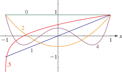
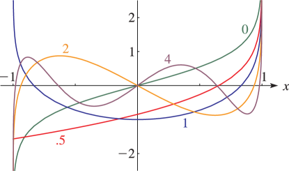
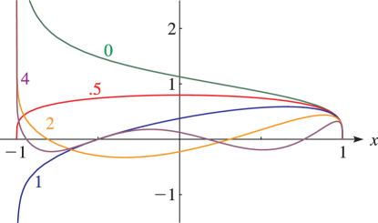
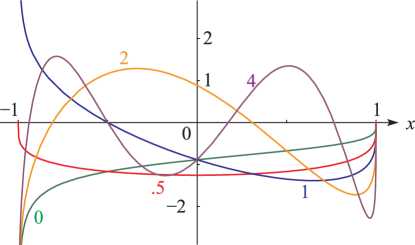
… ►The main functions treated in this chapter are the Legendre functions ${𝖯}_{\nu }\left(x\right)$, ${𝖰}_{\nu }\left(x\right)$, $P_{\nu }\left(z\right)$, $Q_{\nu }\left(z\right)$; Ferrers functions ${𝖯}_{\nu }^{\mu }\left(x\right)$, ${𝖰}_{\nu }^{\mu }\left(x\right)$ (also known as the Legendre functions on the cut); associated Legendre functions $P_{\nu }^{\mu }\left(z\right)$, $Q_{\nu }^{\mu }\left(z\right)$, ${𝑸}_{\nu }^{\mu }\left(z\right)$; conical functions ${𝖯}_{-\frac{1}{2}+\mathrm{i}\tau }^{\mu }\left(x\right)$, ${𝖰}_{-\frac{1}{2}+\mathrm{i}\tau }^{\mu }\left(x\right)$, ${\widehat{𝖰}}_{-\frac{1}{2}+\mathrm{i}\tau }^{\mu }\left(x\right)$, $P_{-\frac{1}{2}+\mathrm{i}\tau }^{\mu }\left(x\right)$, $Q_{-\frac{1}{2}+\mathrm{i}\tau }^{\mu }\left(x\right)$ (also known as Mehler functions). … ►Among other notations commonly used in the literature Erdélyi et al. (1953a) and Olver (1997b) denote ${𝖯}_{\nu }^{\mu }\left(x\right)$ and ${𝖰}_{\nu }^{\mu }\left(x\right)$ by ${\mathrm{P}}_{\nu }^{\mu }(x)$ and ${\mathrm{Q}}_{\nu }^{\mu }(x)$, respectively. Magnus et al. (1966) denotes ${𝖯}_{\nu }^{\mu }\left(x\right)$, ${𝖰}_{\nu }^{\mu }\left(x\right)$, $P_{\nu }^{\mu }\left(z\right)$, and $Q_{\nu }^{\mu }\left(z\right)$ by $P_{\nu }^{\mu }(x)$, $Q_{\nu }^{\mu }(x)$, ${𝔓}_{\nu }^{\mu }(z)$, and ${𝔔}_{\nu }^{\mu }(z)$, respectively. Hobson (1931) denotes both ${𝖯}_{\nu }^{\mu }\left(x\right)$ and $P_{\nu }^{\mu }\left(x\right)$ by $P_{\nu }^{\mu }\left(x\right)$; similarly for ${𝖰}_{\nu }^{\mu }\left(x\right)$ and $Q_{\nu }^{\mu }\left(x\right)$.