of%20one%20variable

SearchAdvancedHelp

(0.004 seconds)

1—10 of 30 matching pages

1: Bibliography F

… ►

ⓘ

Notes:

The “Freely Distributable LIBM” package provides implementations of standard elementary functions plus a few higher functions, e.g. gamma. Double precision, maximum accuracy 20S. Developed by Sun Microsystems.

External Links:

GAMS (package FDLIBM)

Referenced by:

§ ‣ Software Cross Index, § ‣ Software Cross Index.

Encodings:

BibTeX

… ►

Sur certaines sommes des intégral-cosinus. Bull. Soc. Math. Phys. Serbie 12, pp. 13–20 (French).

ⓘ

External Links:

MathReview (L. Carlitz), ZentralBlatt

Referenced by:

§6.15.

Encodings:

BibTeX

►

The third Appell function for one large variable. J. Approx. Theory 165, pp. 60–69.

ⓘ

External Links:

ISSN 0021-9045, Document, FullText, MathReview Entry, ZentralBlatt

Referenced by:

§16.13, §16.13.

Encodings:

BibTeX

… ►

The second Appell function for one large variable. Mediterr. J. Math. 10 (4), pp. 1853–1865.

ⓘ

External Links:

ISSN 1660-5446, Document, FullText, MathReview Entry, ZentralBlatt

Referenced by:

§16.13, §16.13.

Encodings:

BibTeX

… ►

On weighted polynomial approximation on the whole real axis. Acta Math. Acad. Sci. Hungar. 20, pp. 223–225.

ⓘ

External Links:

ISSN 0001-5954, Document, Link, MathReview (A. K. Varma)

Referenced by:

§18.32.

Encodings:

BibTeX

…

2: 18.40 Methods of Computation

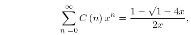
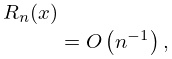
… ►The problem of moments is simply stated and the early work of Stieltjes, Markov, and Chebyshev on this problem was the origin of the understanding of the importance of both continued fractions and OP’s in many areas of analysis. … ►See Gautschi (1983) for examples of numerically stable and unstable use of the above recursion relations, and how one can then usefully differentiate between numerical results of low and high precision, as produced thereby. 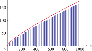… ►Results of low ($2$ to $3$ decimal digits) precision for $w(x)$ are easily obtained for $N\sim 10$ to $20$. Gautschi (2004, p. 119–120) has explored the $\epsilon \to 0^{+}$ limit via the Wynn $\epsilon$-algorithm, (3.9.11) to accelerate convergence, finding four to eight digits of precision in $w(x)$, depending smoothly on $x^{\prime }$, for $N\approx 4000$, for an example involving first numerator Legendre OP’s. … ►This is a challenging case as the desired $w^{\mathrm{RCP}}(x)$ on $[-1,1]$ has an essential singularity at $x=-1$. …

3: 23.9 Laurent and Other Power Series

… ►

$c_2={\displaystyle \frac{1}{20}}{g}_2,$

►

$c_3={\displaystyle \frac{1}{28}}{g}_3,$

… ►For $j=1,2,3$, and with $e_j$ as in §23.3(i), ►

23.9.6 $$\mathrm{\wp }\left({\omega }_j+t\right)=e_j+(3{e_j}^2-5c_2)t^2+(10c_2{e}_j+21c_3)t^4+(7c_2{e_j}^2+21c_3{e}_j+5c_2^2)t^6+O\left(t^8\right),$$

ⓘ

Symbols:

$O\left(x\right)$: order not exceeding, $\mathrm{\wp }\left(z\right)$ (= $\mathrm{\wp }\left(z|𝕃\right)$ = $\mathrm{\wp }(z;g_2,g_3)$): Weierstrass $\mathrm{\wp }$-function, $e_j$: Weierstrass lattice roots, $𝕃$: lattice, ${\omega }_1$, ${\omega }_3$, ${\omega }_2=-{\omega }_1-{\omega }_3$: lattice generators, $c_n$ and $t$: variable

Referenced by:

§23.9

Permalink:

http://dlmf.nist.gov/23.9.E6

Encodings:

pMML, png, TeX

See also:

Annotations for §23.9 and Ch.23

… ►Also, Abramowitz and Stegun (1964, (18.5.25)) supplies the first 22 terms in the reverted form of (23.9.2) as $1/\mathrm{\wp }\left(z\right)\to 0$. …

4: 7.23 Tables

… ►

§7.23(ii) Real Variables

… ►

§7.23(iii) Complex Variables, $z=x+\mathrm{i}y$

… ►

Zhang and Jin (1996, pp. 638, 640–641) includes the real and imaginary parts of $\mathrm{erf}z$, $x\in [0,5]$, $y=0.5(.5)3$, 7D and 8D, respectively; the real and imaginary parts of ${\int }_x^{\mathrm{\infty }}{\mathrm{e}}^{\pm \mathrm{i}{t}^2}dt$, $(1/\sqrt{\pi }){\mathrm{e}}^{\mp \mathrm{i}(x^2+(\pi /4))}{\int }_x^{\mathrm{\infty }}{\mathrm{e}}^{\pm \mathrm{i}{t}^2}dt$, $x=0(.5)20(1)25$, 8D, together with the corresponding modulus and phase to 8D and 6D (degrees), respectively.

… ►

Fettis et al. (1973) gives the first 100 zeros of $\mathrm{erf}z$ and $w\left(z\right)$ (the table on page 406 of this reference is for $w\left(z\right)$, not for $\mathrm{erfc}z$), 11S.

…

5: Bibliography O

… ►

An error analysis of the modified Clenshaw method for evaluating Chebyshev and Fourier series. J. Inst. Math. Appl. 20 (3), pp. 379–391.

ⓘ

External Links:

Document, MathReview (David L. Elliott), ZentralBlatt

Referenced by:

§3.11(ii).

Encodings:

BibTeX

… ►

Note on backward recurrence algorithms. Math. Comp. 26 (120), pp. 941–947.

ⓘ

External Links:

FullText, MathReview (Walter Gautschi), ZentralBlatt

Referenced by:

§10.74(iv), §3.6(v).

Encodings:

BibTeX

… ►

On the asymptotic solution of second-order differential equations having an irregular singularity of rank one, with an application to Whittaker functions. J. Soc. Indust. Appl. Math. Ser. B Numer. Anal. 2 (2), pp. 225–243.

ⓘ

External Links:

Document, MathReview (T. E. Hull), ZentralBlatt

Referenced by:

§13.19, §13.7(ii).

Encodings:

BibTeX

… ►

OEIS Foundation, Inc., Highland Park, New Jersey.

ⓘ

Notes:

A tool for finding and identifying integer sequences.

External Links:

On-Line Encyclopedia of Integer Sequences

Referenced by:

5th item.

Encodings:

BibTeX

… ►

Numerical Computing with IEEE Floating Point Arithmetic. Society for Industrial and Applied Mathematics (SIAM), Philadelphia, PA.

ⓘ

Notes:

Including one theorem, one rule of thumb, and one hundred and one exercises

External Links:

ISBN 0-89871-482-6, MathReview (Jesse L. Barlow), ZentralBlatt

Referenced by:

§3.1(i).

Encodings:

BibTeX

6: 10.73 Physical Applications

… ►and on separation of variables we obtain solutions of the form ${\mathrm{e}}^{\pm \mathrm{i}n\varphi }{\mathrm{e}}^{\pm \kappa z}{J}_n\left(\kappa r\right)$, from which a solution satisfying prescribed boundary conditions may be constructed. … ►on assuming a time dependence of the form ${\mathrm{e}}^{\pm \mathrm{i}kt}$. …See Krivoshlykov (1994, Chapter 2, §2.2.10; Chapter 5, §5.2.2), Kapany and Burke (1972, Chapters 4–6; Chapter 7, §A.1), and Slater (1942, Chapter 4, §§20, 25). … ►On separation of variables into cylindrical coordinates, the Bessel functions $J_n\left(x\right)$, and modified Bessel functions $I_n\left(x\right)$ and $K_n\left(x\right)$, all appear. … ►With the spherical harmonic $Y_{\mathrm{\ell },m}\left(\theta ,\varphi \right)$ defined as in §14.30(i), the solutions are of the form $f=g_{\mathrm{\ell }}(k\rho )Y_{\mathrm{\ell },m}\left(\theta ,\varphi \right)$ with $g_{\mathrm{\ell }}={𝗃}_{\mathrm{\ell }}$, ${𝗒}_{\mathrm{\ell }}$, ${𝗁}_{\mathrm{\ell }}^{(1)}$, or ${𝗁}_{\mathrm{\ell }}^{(2)}$, depending on the boundary conditions. …

7: Bibliography C

… ►

A note on Euler numbers and polynomials. Nagoya Math. J. 7, pp. 35–43.

ⓘ

External Links:

MathReview (A. L. Whiteman), ZentralBlatt

Referenced by:

§24.10(iv).

Encodings:

BibTeX

… ►

On computing elliptic integrals and functions. J. Math. and Phys. 44, pp. 36–51.

ⓘ

External Links:

MathReview (R. Nicolovius), ZentralBlatt

Referenced by:

§19.36(ii), §19.36(ii).

Encodings:

BibTeX

… ►

Asymptotic estimates for generalized Stirling numbers. Analysis (Munich) 20 (1), pp. 1–13.

ⓘ

External Links:

ISSN 0174-4747, MathReview (F. T. Howard), ZentralBlatt

Referenced by:

§26.8(vii).

Encodings:

BibTeX

… ►

Validated computation of certain hypergeometric functions. ACM Trans. Math. Software 38 (2), pp. Art. 11, 20.

ⓘ

External Links:

ISSN 0098-3500, Document, FullText, MathReview Entry, ZentralBlatt

Referenced by:

§13.29(v), §15.19(v).

Encodings:

BibTeX

… ►

Coulomb effects in the Klein-Gordon equation for pions. Phys. Rev. C 20 (2), pp. 696–704.

ⓘ

External Links:

Document

Referenced by:

5th item.

Encodings:

BibTeX

…

8: 26.5 Lattice Paths: Catalan Numbers

… ►It counts the number of lattice paths from $(0,0)$ to $(n,n)$ that stay on or above the line $y=x$. … ►

Table 26.5.1: Catalan numbers.

► ►►►

$n$	$C\left(n\right)$	$n$	$C\left(n\right)$	$n$	$C\left(n\right)$
…
6	132	13	7 42900	20	65641 20420

►

… ►

26.5.2 $$\sum _{n=0}^{\mathrm{\infty }}C\left(n\right)x^n=\frac{1-\sqrt{1-4x}}{2x},$$ .

ⓘ

Symbols:

$C\left(n\right)$: Catalan number, $x$: real variable and $n$: nonnegative integer

Permalink:

http://dlmf.nist.gov/26.5.E2

Encodings:

pMML, png, TeX

See also:

Annotations for §26.5(ii), §26.5 and Ch.26

…

9: 6.16 Mathematical Applications

… ►

6.16.1

ⓘ

Symbols:

$\pi$: the ratio of the circumference of a circle to its diameter, $\sin z$: sine function and $x$: real variable

Permalink:

http://dlmf.nist.gov/6.16.E1

Encodings:

pMML, png, TeX

See also:

Annotations for §6.16(i), §6.16 and Ch.6

… ►

6.16.4 $$R_n(x)=O\left(n^{-1}\right),$$ $n\to \mathrm{\infty }$,

ⓘ

Symbols:

$O\left(x\right)$: order not exceeding, $x$: real variable, $n$: nonnegative integer and $R_n(x)$: remainder term

Permalink:

http://dlmf.nist.gov/6.16.E4

Encodings:

pMML, png, TeX

See also:

Annotations for §6.16(i), §6.16 and Ch.6

… ►Similarly if $x=\pi /n$, then the limiting value of $S_n(x)$ undershoots $\frac{1}{4}\pi$ by approximately 10%, and so on. … ►

6.16.5 $$\mathrm{li}\left(x\right)-\pi (x)=O\left(\sqrt{x}\ln x\right),$$ $x\to \mathrm{\infty }$,

ⓘ

Symbols:

$O\left(x\right)$: order not exceeding, $\mathrm{li}\left(x\right)$: logarithmic integral, $\ln z$: principal branch of logarithm function, $x$: real variable and $\pi (x)$: number of primes $\le x$

A&S Ref:

5.1.50

Permalink:

http://dlmf.nist.gov/6.16.E5

Encodings:

pMML, png, TeX

See also:

Annotations for §6.16(ii), §6.16 and Ch.6

… ►

►►

Figure 6.16.2: The logarithmic integral $\mathrm{li}\left(x\right)$, together with vertical bars indicating the value of $\pi (x)$ for $x=10,20,\mathrm{\dots },1000$. Magnify

10: 5.11 Asymptotic Expansions

… ►

5.11.1 $$\mathrm{Ln}\mathrm{\Gamma }\left(z\right)\sim \left(z-\frac{1}{2}\right)\ln z-z+\frac{1}{2}\ln \left(2\pi \right)+\sum _{k=1}^{\mathrm{\infty }}\frac{B_{2k}}{2k(2k-1)z^{2k-1}}$$

ⓘ

Symbols:

$B_n$: Bernoulli numbers, $\mathrm{\Gamma }\left(z\right)$: gamma function, $\sim$: Poincaré asymptotic expansion, $\pi$: the ratio of the circumference of a circle to its diameter, $\mathrm{Ln}z$: general logarithm function, $\ln z$: principal branch of logarithm function, $k$: nonnegative integer and $z$: complex variable

A&S Ref:

6.1.40

Referenced by:

§5.11(i), §5.11(i), §5.11(ii), §5.11(ii), Erratum (V1.0.10) for Equations (5.9.10), (5.9.11), (5.10.1), (5.11.1), (5.11.8)

Permalink:

http://dlmf.nist.gov/5.11.E1

Encodings:

pMML, png, TeX

Addition (effective with 1.0.10):

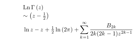
To increase the region of validity of this equation, the logarithm of the gamma function that appears on its left-hand side has been changed to $\mathrm{Ln}\mathrm{\Gamma }\left(z\right)$, where $\mathrm{Ln}$ is the general logarithm. Originally $\ln \mathrm{\Gamma }\left(z\right)$ was used, where $\ln$ is the principal branch of the logarithm.

Suggested 2015-02-13 by Philippe Spindel

See also:

Annotations for §5.11(i), §5.11 and Ch.5

… ►Wrench (1968) gives exact values of $g_k$ up to $g_{20}$. … ►

5.11.8 $$\mathrm{Ln}\mathrm{\Gamma }\left(z+h\right)\sim \left(z+h-\frac{1}{2}\right)\ln z-z+\frac{1}{2}\ln \left(2\pi \right)+\sum _{k=2}^{\mathrm{\infty }}\frac{{(-1)}^k{B}_k\left(h\right)}{k(k-1)z^{k-1}},$$

ⓘ

Symbols:

$B_n\left(x\right)$: Bernoulli polynomials, $\mathrm{\Gamma }\left(z\right)$: gamma function, $\sim$: Poincaré asymptotic expansion, $\pi$: the ratio of the circumference of a circle to its diameter, $[a,b]$: closed interval, $\mathrm{Ln}z$: general logarithm function, $\ln z$: principal branch of logarithm function, $k$: nonnegative integer and $z$: complex variable

Referenced by:

§12.10(ii), (5.11.8), §5.11(i), §5.11(ii), Erratum (V1.0.10) for Equations (5.9.10), (5.9.11), (5.10.1), (5.11.1), (5.11.8), Erratum (V1.0.11) for Equation (5.11.8)

Permalink:

http://dlmf.nist.gov/5.11.E8

Encodings:

pMML, png, TeX

Generalization (effective with 1.0.11):

Originally $h$ in (5.11.8) was unnecessarily restricted to lie in the interval $[0,1]$. In fact, $h$ may lie anywhere in the complex plane.

Suggested 2015-02-28 by Nico Temme

Addition (effective with 1.0.10):

To increase the region of validity of this equation, the logarithm of the gamma function that appears on its left-hand side has been changed to $\mathrm{Ln}\mathrm{\Gamma }\left(z+h\right)$, where $\mathrm{Ln}$ is the general logarithm. Originally $\ln \mathrm{\Gamma }\left(z+h\right)$ was used, where $\ln$ is the principal branch of the logarithm.

Suggested 2015-02-13 by Philippe Spindel

See also:

Annotations for §5.11(i), §5.11(i), §5.11 and Ch.5

… ►

5.11.12 $$\frac{\mathrm{\Gamma }\left(z+a\right)}{\mathrm{\Gamma }\left(z+b\right)}\sim z^{a-b},$$

ⓘ

Symbols:

$\mathrm{\Gamma }\left(z\right)$: gamma function, $\sim$: asymptotic equality, $z$: complex variable, $a$: real or complex variable and $b$: real or complex variable

Referenced by:

§5.11(i)

Permalink:

http://dlmf.nist.gov/5.11.E12

Encodings:

pMML, png, TeX

See also:

Annotations for §5.11(iii), §5.11 and Ch.5

►

5.11.13 $$\frac{\mathrm{\Gamma }\left(z+a\right)}{\mathrm{\Gamma }\left(z+b\right)}\sim z^{a-b}\sum _{k=0}^{\mathrm{\infty }}\frac{G_k(a,b)}{z^k},$$

ⓘ

Symbols:

$\mathrm{\Gamma }\left(z\right)$: gamma function, $\sim$: Poincaré asymptotic expansion, $k$: nonnegative integer, $z$: complex variable, $a$: real or complex variable, $b$: real or complex variable and $G_k(a,b)$: coefficients

A&S Ref:

6.1.47

Permalink:

http://dlmf.nist.gov/5.11.E13

Encodings:

pMML, png, TeX

See also:

Annotations for §5.11(iii), §5.11 and Ch.5

…