of%20imaginary%20order

SearchAdvancedHelp

(0.002 seconds)

1—10 of 15 matching pages

1: 10.75 Tables

… ►

Zhang and Jin (1996, pp. 185–195) tabulates $J_n\left(x\right)$, $J_n^{\prime }\left(x\right)$, $Y_n\left(x\right)$, $Y_n^{\prime }\left(x\right)$, $n=0(1)10(10)50,100$, $x=1$, 5, 10, 25, 50, 100, 9S; $J_{n+\alpha }\left(x\right)$, $J_{n+\alpha }^{\prime }\left(x\right)$, $Y_{n+\alpha }\left(x\right)$, $Y_{n+\alpha }^{\prime }\left(x\right)$, $n=0(1)5,10,30,50,100$, $\alpha =\frac{1}{4},\frac{1}{3},\frac{1}{2},\frac{2}{3},\frac{3}{4}$, $x=1,5,10,50$, 8S; real and imaginary parts of $J_{n+\alpha }\left(z\right)$, $J_{n+\alpha }^{\prime }\left(z\right)$, $Y_{n+\alpha }\left(z\right)$, $Y_{n+\alpha }^{\prime }\left(z\right)$, $n=0(1)15,20(10)50,100$, $\alpha =0,\frac{1}{2}$, $z=4+2\mathrm{i}$, $20+10\mathrm{i}$, 8S.

… ►

MacDonald (1989) tabulates the first 30 zeros, in ascending order of absolute value in the fourth quadrant, of the function $J_0\left(z\right)-\mathrm{i}{J}_1\left(z\right)$, 6D. (Other zeros of this function can be obtained by reflection in the imaginary axis).

… ►

Zhang and Jin (1996, pp. 240–250) tabulates $I_n\left(x\right)$, $I_n^{\prime }\left(x\right)$, $K_n\left(x\right)$, $K_n^{\prime }\left(x\right)$, $n=0(1)10(10)50,100$, $x=1,5,10,25,50,100$, 9S; $I_{n+\alpha }\left(x\right)$, $I_{n+\alpha }^{\prime }\left(x\right)$, $K_{n+\alpha }\left(x\right)$, $K_{n+\alpha }^{\prime }\left(x\right)$, $n=0(1)5$, 10, 30, 50, 100, $\alpha =\frac{1}{4}$, $\frac{1}{3}$, $\frac{1}{2}$, $\frac{2}{3}$, $\frac{3}{4}$, $x=1$, 5, 10, 50, 8S; real and imaginary parts of $I_{n+\alpha }\left(z\right)$, $I_{n+\alpha }^{\prime }\left(z\right)$, $K_{n+\alpha }\left(z\right)$, $K_{n+\alpha }^{\prime }\left(z\right)$, $n=0(1)15$, 20(10)50, 100, $\alpha =0,\frac{1}{2}$, $z=4+2\mathrm{i},20+10\mathrm{i}$, 8S.

… ►

§10.75(viii) Modified Bessel Functions of Imaginary or Complex Order

… ►

Žurina and Karmazina (1967) tabulates ${\tilde{K}}_{\nu }\left(x\right)$ for $\nu =0.01(.01)10$, $x=0.1(.1)10.2$, 7S.

…

2: 10.3 Graphics

… ►

§10.3(i) Real Order and Variable

… ►

§10.3(ii) Real Order, Complex Variable

… ►

§10.3(iii) Imaginary Order, Real Variable

… ►

►►

Figure 10.3.18: ${\tilde{J}}_1\left(x\right)$, ${\tilde{Y}}_1\left(x\right)$, $0.01\le x\le 10$. Magnify

►

►►

Figure 10.3.19: ${\tilde{J}}_5\left(x\right)$, ${\tilde{Y}}_5\left(x\right)$, $0.01\le x\le 10$. Magnify

3: Bibliography D

… ►

A simplified algorithm for the second-order sound fields. J. Acoust. Soc. Amer. 108 (6), pp. 2759–2764.

ⓘ

External Links:

Document

Referenced by:

§8.24(iii).

Encodings:

BibTeX

… ►

Complex zeros of cylinder functions. Math. Comp. 20 (94), pp. 215–222.

ⓘ

Notes:

For a numerical error in one of the zeros see Amos (1985).

External Links:

ISSN 0025-5718, FullText, MathReview, ZentralBlatt

Referenced by:

2nd item.

Encodings:

BibTeX

… ►

Uniform asymptotic expansions for Whittaker’s confluent hypergeometric functions. SIAM J. Math. Anal. 20 (3), pp. 744–760.

ⓘ

Notes:

(This reference has several typographical errors.)

External Links:

ISSN 0036-1410, Document, MathReview (F. W. J. Olver), ZentralBlatt

Referenced by:

§13.21(ii), §13.21(iii), §13.21(iv).

Encodings:

BibTeX

►

Bessel functions of purely imaginary order, with an application to second-order linear differential equations having a large parameter. SIAM J. Math. Anal. 21 (4), pp. 995–1018.

ⓘ

Notes:

Errata: In eq. (2.8) replace ${(x^2/4)}^2$ by ${(x^2/4)}^s$. In eq. (4.2) $\varphi (\zeta )$ should be replaced by $\psi (\zeta )$. In the second line of eq. (4.7) insert an external factor $e^{-2\pi ij/3}$ and change the upper limit of the sum to $n-1$. In eq. (4.15) the factor $\zeta$ is missing from the arguments of the functions Bi_ν and Bi’_ν.

External Links:

ISSN 0036-1410, Document, MathReview (A. de Castro Brzezicki), ZentralBlatt

Referenced by:

§10.24, §10.45, §2.8(iv).

Encodings:

BibTeX

… ►

Conical functions of purely imaginary order and argument. Proc. Roy. Soc. Edinburgh Sect. A 143 (5), pp. 929–955.

ⓘ

External Links:

ISSN 0308-2105, Document, Link, MathReview (Eugenia N. Petropoulou), ZentralBlatt

Referenced by:

§14.20(ix), §14.20(ix).

Encodings:

BibTeX

…

4: 18.40 Methods of Computation

… ►It is now necessary to take the limit $\epsilon \to 0+$ of $F(x^{\prime }+\mathrm{i}\epsilon )$, and the imaginary part is the required Stieltjes–Perron inversion: ►

18.40.6 $$\underset{\epsilon \to 0+}{lim}{\int }_a^b\frac{w(x)dx}{x^{\prime }+\mathrm{i}\epsilon -x}dx={⨍}_a^b\frac{w(x)dx}{x^{\prime }-x}-\mathrm{i}\pi w(x^{\prime }),$$

ⓘ

Symbols:

$dx$: differential of $x$ , $\mathrm{i}$: imaginary unit, $\int$: integral, ${⨍}_a^b$: Cauchy principal value, $w(x)$: weight function and $x$: real variable

Permalink:

http://dlmf.nist.gov/18.40.E6

Encodings:

pMML, png, TeX

See also:

Annotations for §18.40(ii), §18.40(ii), §18.40 and Ch.18

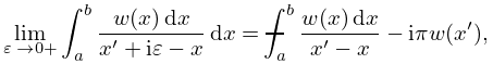
►The question is then: how is this possible given only $F_N(z)$, rather than $F(z)$ itself? $F_N(z)$ often converges to smooth results for $z$ off the real axis for $\mathrm{\Im }z$ at a distance greater than the pole spacing of the $x_n$, this may then be followed by approximate numerical analytic continuation via fitting to lower order continued fractions (either Padé, see §3.11(iv), or pointwise continued fraction approximants, see Schlessinger (1968, Appendix)), to $F_N(z)$ and evaluating these on the real axis in regions of higher pole density that those of the approximating function. Results of low ($2$ to $3$ decimal digits) precision for $w(x)$ are easily obtained for $N\sim 10$ to $20$. …

5: 11.6 Asymptotic Expansions

… ►

§11.6(ii) Large $|\nu |$, Fixed $z$

►

11.6.5 $${𝐇}_{\nu }\left(z\right),{𝐋}_{\nu }\left(z\right)\sim \frac{z}{\pi \nu \sqrt{2}}{\left(\frac{\mathrm{e}z}{2\nu }\right)}^{\nu },$$ $|\mathrm{ph}\nu |\le \pi -\delta$.

ⓘ

Symbols:

${𝐇}_{\nu }\left(z\right)$: Struve function, $\sim$: asymptotic equality, $\pi$: the ratio of the circumference of a circle to its diameter, $\mathrm{e}$: base of natural logarithm, ${𝐋}_{\nu }\left(z\right)$: modified Struve function, $\mathrm{ph}$: phase, $z$: complex variable, $\nu$: real or complex order and $\delta$: arbitrary small positive constant

Referenced by:

(11.11.7)

Permalink:

http://dlmf.nist.gov/11.6.E5

Encodings:

pMML, png, TeX

See also:

Annotations for §11.6(ii), §11.6 and Ch.11

… ►

11.6.7 $${𝐌}_{\nu }\left(\lambda \nu \right)\sim -\frac{{(\frac{1}{2}\lambda \nu )}^{\nu -1}}{\sqrt{\pi }\mathrm{\Gamma }\left(\nu +\frac{1}{2}\right)}\sum _{k=0}^{\mathrm{\infty }}\frac{k!c_k(\mathrm{i}\lambda )}{{\nu }^k},$$ $|\mathrm{ph}\nu |\le \frac{1}{2}\pi -\delta$.

ⓘ

Symbols:

$\mathrm{\Gamma }\left(z\right)$: gamma function, ${𝐌}_{\nu }\left(z\right)$: modified Struve function, $\sim$: Poincaré asymptotic expansion, $\pi$: the ratio of the circumference of a circle to its diameter, $!$: factorial (as in $n!$), $\mathrm{i}$: imaginary unit, $\mathrm{ph}$: phase, $\nu$: real or complex order, $k$: nonnegative integer, $\delta$: arbitrary small positive constant, $\lambda$: parameter and $c_k(\lambda )$: expansion function

Referenced by:

§11.6(iii)

Permalink:

http://dlmf.nist.gov/11.6.E7

Encodings:

pMML, png, TeX

See also:

Annotations for §11.6(iii), §11.6 and Ch.11

… ►

$c_3(\lambda )=20{\lambda }^{-6}-4{\lambda }^{-4},$

… ►

11.6.9 $${𝐋}_{\nu }\left(\lambda \nu \right)\sim I_{\nu }\left(\lambda \nu \right),$$ $|\mathrm{ph}\nu |\le \frac{1}{2}\pi -\delta$,

ⓘ

Symbols:

$\sim$: asymptotic equality, $\pi$: the ratio of the circumference of a circle to its diameter, $I_{\nu }\left(z\right)$: modified Bessel function of the first kind, ${𝐋}_{\nu }\left(z\right)$: modified Struve function, $\mathrm{ph}$: phase, $\nu$: real or complex order, $\delta$: arbitrary small positive constant and $\lambda$: parameter

Referenced by:

§11.6(iii)

Permalink:

http://dlmf.nist.gov/11.6.E9

Encodings:

pMML, png, TeX

See also:

Annotations for §11.6(iii), §11.6 and Ch.11

…

6: Bibliography B

… ►

Pionic atoms. Annual Review of Nuclear and Particle Science 20, pp. 467–508.

ⓘ

External Links:

Document

Referenced by:

§33.22(iv).

Encodings:

BibTeX

… ►

Asymptotic expansions of the modified Bessel function of the third kind of imaginary order. SIAM J. Appl. Math. 15, pp. 1315–1323.

ⓘ

External Links:

ISSN 0036-1399, Document, MathReview (F. W. J. Olver), ZentralBlatt

Referenced by:

§10.45.

Encodings:

BibTeX

… ►

Coulomb functions (negative energies). Comput. Phys. Comm. 20 (3), pp. 447–458.

ⓘ

Notes:

Double-precision Fortran code.

External Links:

Document, Code

Referenced by:

1st item, 4th item.

Encodings:

BibTeX

… ►

Orthogonality relations for the associated Legendre functions of imaginary order. Integral Transforms Spec. Funct. 24 (4), pp. 331–337.

ⓘ

External Links:

ISSN 1065-2469, Document, FullText, MathReview (Praveen Agarwal), ZentralBlatt

Referenced by:

§14.17(iii), §14.17(iii).

Encodings:

BibTeX

… ►

Bounds and algorithms for the $K$-Bessel function of imaginary order. LMS J. Comput. Math. 16, pp. 78–108.

ⓘ

External Links:

ISSN 1461-1570, Document, MathReview (Jürgen Müller), ZentralBlatt

Referenced by:

§10.45, §10.45.

Encodings:

BibTeX

…

7: Software Index

… ► ►►►►►►►

	Open Source													With Book						Commercial
…
10.77(iii) Bessel Functions–Real Order and Argument	✓	✓	✓	✓	✓	✓		✓	✓		✓	✓	✓		✓	✓	✓	✓	✓	✓	✓	✓	✓	✓	NMS
10.77(iv) Bessel Functions–Integer or Half-Integer Order and Complex Arguments, including Kelvin Functions	✓	✓	✓									a	✓	✓			✓	✓	✓	✓	✓	✓	✓
…
10.77(vi) Bessel Functions–Imaginary Order and Real Argument	✓	✓										✓	✓								✓	✓	✓
10.77(viii) Bessel Functions–Complex Order and Argument	✓	✓										✓	✓								✓	✓	✓
…
20 Theta Functions
…

…

8: 36.5 Stokes Sets

… ►

36.5.4 $$80x^5-40x^4-55x^3+5x^2+20x-1=0,$$

ⓘ

Symbols:

$x$: real parameter

Permalink:

http://dlmf.nist.gov/36.5.E4

Encodings:

pMML, png, TeX

See also:

Annotations for §36.5(ii), §36.5(ii), §36.5 and Ch.36

… ►

36.5.7 $$X=\frac{9}{20}+20u^4-\frac{Y^2}{20u^2}+6u^2\mathrm{sign}\left(z\right),$$

ⓘ

Symbols:

$\mathrm{sign}x$: sign of, $z$: real parameter, $X$: scaled coordinate and $Y$: scaled coordinate

Permalink:

http://dlmf.nist.gov/36.5.E7

Encodings:

pMML, png, TeX

See also:

Annotations for §36.5(ii), §36.5(ii), §36.5 and Ch.36

…

9: 12.11 Zeros

… ►

12.11.1 $$z_{a,s}={\mathrm{e}}^{\frac{3}{4}\pi \mathrm{i}}\sqrt{2{\tau }_s}\left(1-\frac{\mathrm{i}a{\lambda }_s}{2{\tau }_s}+\frac{2a^2{\lambda }_s^2-8a^2{\lambda }_s+4a^2+3}{16{\tau }_s^2}+O\left({\lambda }_s^3{\tau }_s^{-3}\right)\right),$$

ⓘ

Symbols:

$O\left(x\right)$: order not exceeding, $\pi$: the ratio of the circumference of a circle to its diameter, $\mathrm{e}$: base of natural logarithm, $\mathrm{i}$: imaginary unit, $z$: complex variable, $s$: nonnegative integer, $a$: real or complex parameter, ${\tau }_s$ and ${\lambda }_s$

Permalink:

http://dlmf.nist.gov/12.11.E1

Encodings:

pMML, png, TeX

See also:

Annotations for §12.11(ii), §12.11 and Ch.12

… ►

12.11.2 $${\tau }_s=\left(2s+\frac{1}{2}-a\right)\pi +\mathrm{i}\ln \left({\pi }^{-\frac{1}{2}}{2}^{-a-\frac{1}{2}}\mathrm{\Gamma }\left(\frac{1}{2}+a\right)\right),$$

ⓘ

Defines:

${\tau }_s$ (locally)

Symbols:

$\mathrm{\Gamma }\left(z\right)$: gamma function, $\pi$: the ratio of the circumference of a circle to its diameter, $\mathrm{i}$: imaginary unit, $\ln z$: principal branch of logarithm function, $s$: nonnegative integer and $a$: real or complex parameter

Permalink:

http://dlmf.nist.gov/12.11.E2

Encodings:

pMML, png, TeX

See also:

Annotations for §12.11(ii), §12.11 and Ch.12

… ►

12.11.3 $${\lambda }_s=\ln {\tau }_s-\frac{1}{2}\pi \mathrm{i}.$$

ⓘ

Defines:

${\lambda }_s$ (locally)

Symbols:

$\pi$: the ratio of the circumference of a circle to its diameter, $\mathrm{i}$: imaginary unit, $\ln z$: principal branch of logarithm function, $s$: nonnegative integer and ${\tau }_s$

Permalink:

http://dlmf.nist.gov/12.11.E3

Encodings:

pMML, png, TeX

See also:

Annotations for §12.11(ii), §12.11 and Ch.12

… ►For example, let the $s$th real zeros of $U(a,x)$ and $U^{\prime }(a,x)$, counted in descending order away from the point $z=2\sqrt{-a}$, be denoted by $u_{a,s}$ and $u_{a,s}^{\prime }$, respectively. … ►

12.11.9 $$u_{a,1}\sim 2^{\frac{1}{2}}\mu \left(1-\mathrm{1.85575\hspace{0.33em}708}{\mu }^{-4/3}-\mathrm{0.34438\hspace{0.33em}34}{\mu }^{-8/3}-\mathrm{0.16871\hspace{0.33em}5}{\mu }^{-4}-0.11414{\mu }^{-16/3}-0.0808{\mu }^{-20/3}-\mathrm{\cdots }\right),$$

ⓘ

Symbols:

$\sim$: Poincaré asymptotic expansion, $a$: real or complex parameter and $u_{a,s}$: zeros

Referenced by:

§12.11(iii)

Permalink:

http://dlmf.nist.gov/12.11.E9

Encodings:

pMML, png, TeX

See also:

Annotations for §12.11(iii), §12.11 and Ch.12

…

10: Bibliography G

… ►

Evaluation of the modified Bessel function of the third kind of imaginary orders. J. Comput. Phys. 175 (2), pp. 398–411.

ⓘ

External Links:

ISSN 0021-9991, Document, MathReview (J. P. Singhal), ZentralBlatt

Referenced by:

§10.74(viii).

Encodings:

BibTeX

►

Computation of the modified Bessel function of the third kind of imaginary orders: Uniform Airy-type asymptotic expansion. J. Comput. Appl. Math. 153 (1-2), pp. 225–234.

ⓘ

External Links:

ISSN 0377-0427, Document, MathReview, ZentralBlatt

Referenced by:

§10.45, §10.74(viii).

Encodings:

BibTeX

… ►

Algorithm 831: Modified Bessel functions of imaginary order and positive argument. ACM Trans. Math. Software 30 (2), pp. 159–164.

ⓘ

External Links:

ISSN 0098-3500, Document, GAMS (module 831; package TOMS), MathReview Entry, ZentralBlatt

Referenced by:

1st item.

Encodings:

BibTeX

►

Computing solutions of the modified Bessel differential equation for imaginary orders and positive arguments. ACM Trans. Math. Software 30 (2), pp. 145–158.

ⓘ

External Links:

ISSN 0098-3500, Document, MathReview, ZentralBlatt

Referenced by:

§10.74(viii).

Encodings:

BibTeX

… ►

Algorithm 939: computation of the Marcum Q-function. ACM Trans. Math. Softw. 40 (3), pp. 20:1–20:21.

ⓘ

Notes:

Includes Fortran program claiming 12S accuracy

External Links:

ISSN 0098-3500, Link, Document, MathReview Entry, ZentralBlatt

Referenced by:

3rd item, §10.77(ix).

Encodings:

BibTeX

…