of%20a%20complex%20variable

SearchAdvancedHelp

(0.009 seconds)

1—10 of 32 matching pages

1: 15.10 Hypergeometric Differential Equation

… ►It has regular singularities at $z=0,1,\mathrm{\infty }$, with corresponding exponent pairs $\{0,1-c\}$, $\{0,c-a-b\}$, $\{a,b\}$, respectively. … ►Moreover, in (15.10.9) and (15.10.10) the symbols $a$ and $b$ are interchangeable. ►(c) If the parameter $c$ in the differential equation equals $2-n=0,-1,-2,\mathrm{\dots }$, then fundamental solutions in the neighborhood of $z=0$ are given by $z^{n-1}$ times those in (a) and (b), with $a$ and $b$ replaced throughout by $a+n-1$ and $b+n-1$, respectively. … ►(e) Finally, if $a-b+1$ equals $n=1,2,3,\mathrm{\dots }$, or $2-n=0,-1,-2,\mathrm{\dots }$, then fundamental solutions in the neighborhood of $z=\mathrm{\infty }$ are given by $z^{-a}$ times those in (a), (b), and (c) with $b$ and $z$ replaced by $a-c+1$ and $1/z$, respectively. … ►The $\left(\genfrac{}{}{0.0pt}{}{6}{3}\right)=20$ connection formulas for the principal branches of Kummer’s solutions are: …

2: 25.11 Hurwitz Zeta Function

… ► $\zeta (s,a)$ has a meromorphic continuation in the $s$-plane, its only singularity in $ℂ$ being a simple pole at $s=1$ with residue $1$. As a function of $a$, with $s$ ($\ne 1$) fixed, $\zeta (s,a)$ is analytic in the half-plane $\mathrm{\Re }a>0$. … ►Most references treat real $a$ with . … ►

$a$-Derivative

… ►When $a=1$, (25.11.35) reduces to (25.2.3). …

3: 25.12 Polylogarithms

… ►In the complex plane ${\mathrm{Li}}_2\left(z\right)$ has a branch point at $z=1$. … ►For real or complex $s$ and $z$ the polylogarithm ${\mathrm{Li}}_s\left(z\right)$ is defined by … ►For each fixed complex $s$ the series defines an analytic function of $z$ for . … ►valid when $\mathrm{\Re }s>0$, $\mathrm{\Im }a>0$ or $\mathrm{\Re }s>1$, $\mathrm{\Im }a=0$. … ►For a uniform asymptotic approximation for $F_s(x)$ see Temme and Olde Daalhuis (1990).

4: 12.11 Zeros

… ►If $a>-\frac{1}{2}$, then $V(a,x)$ has no positive real zeros, and if $a=\frac{3}{2}-2n$, $n\in \mathbb{Z}$, then $V(a,x)$ has a zero at $x=0$. ►

§12.11(ii) Asymptotic Expansions of Large Zeros

►When $a>-\frac{1}{2}$, $U(a,z)$ has a string of complex zeros that approaches the ray $\mathrm{ph}z=\frac{3}{4}\pi$ as $z\to \mathrm{\infty }$, and a conjugate string. When $a>-\frac{1}{2}$ the zeros are asymptotically given by $z_{a,s}$ and $\overline{z_{a,s}}$, where $s$ is a large positive integer and … ►For large negative values of $a$ the real zeros of $U(a,x)$, $U^{\prime }(a,x)$, $V(a,x)$, and $V^{\prime }(a,x)$ can be approximated by reversion of the Airy-type asymptotic expansions of §§12.10(vii) and 12.10(viii). …

5: Bibliography B

… ►

Pionic atoms. Annual Review of Nuclear and Particle Science 20, pp. 467–508.

ⓘ

External Links:

Document

Referenced by:

§33.22(iv).

Encodings:

BibTeX

… ►

A program for computing the Riemann zeta function for complex argument. Comput. Phys. Comm. 20 (3), pp. 441–445.

ⓘ

Notes:

Double-precision Fortran, maximum accuracy 10S.

External Links:

Document, Code, ZentralBlatt

Referenced by:

1st item.

Encodings:

BibTeX

… ►

Coulomb functions (negative energies). Comput. Phys. Comm. 20 (3), pp. 447–458.

ⓘ

Notes:

Double-precision Fortran code.

External Links:

Document, Code

Referenced by:

1st item, 4th item.

Encodings:

BibTeX

… ►

A short table of the functions ${\mathrm{Ki}}_n(x)$, from $n=1$ to $n=16$ . Phil. Mag. Series 7 20, pp. 343–347.

ⓘ

External Links:

Document, ZentralBlatt

Referenced by:

§10.43(iii), 2nd item.

Encodings:

BibTeX

… ►

Several Complex Variables. Princeton Mathematical Series, Vol. 10, Princeton University Press, Princeton, N.J..

ⓘ

External Links:

MathReview (P. Thullen), ZentralBlatt

Referenced by:

§35.2.

Encodings:

BibTeX

…

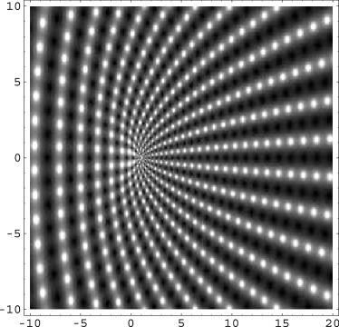
6: 22.3 Graphics

… ►

§22.3(i) Real Variables: Line Graphs

… ►

§22.3(ii) Real Variables: Surfaces

… ►

§22.3(iii) Complex $z$; Real $k$

… ►

§22.3(iv) Complex $k$

… ►

►►

Figure 22.3.28: Density plot of $|\mathrm{sn}(20,k)|$ as a function of complex $k^2$, $-10\le \mathrm{\Re }\left(k^2\right)\le 20$, $-10\le \mathrm{\Im }\left(k^2\right)\le 10$. … Magnify

…

7: Bibliography C

… ►

Analytical solution of a model for complex food webs. Phys. Rev. E 65 (3), pp. (030901–1)–(030901–4).

ⓘ

External Links:

Document

Referenced by:

§8.24(i).

Encodings:

BibTeX

… ►

Approximations and Complex Multiplication According to Ramanujan. In Ramanujan Revisited (Urbana-Champaign, Ill., 1987), G. E. Andrews, R. A. Askey, B. C. Bernd, K. G. Ramanathan, and R. A. Rankin (Eds.), pp. 375–472.

ⓘ

External Links:

MathReview (Maurice Mignotte), ZentralBlatt

Referenced by:

§20.11(iii).

Encodings:

BibTeX

… ►

Algorithm 714: CELEFUNT – A portable test package for complex elementary functions. ACM Trans. Math. Software 19 (1), pp. 1–21.

ⓘ

External Links:

ISSN 0098-3500, Document, GAMS (module 714; package TOMS), ZentralBlatt

Referenced by:

1st item.

Encodings:

BibTeX

… ►

Validated computation of certain hypergeometric functions. ACM Trans. Math. Software 38 (2), pp. Art. 11, 20.

ⓘ

External Links:

ISSN 0098-3500, Document, FullText, MathReview Entry, ZentralBlatt

Referenced by:

§13.29(v), §15.19(v).

Encodings:

BibTeX

… ►

An Introduction to the Theory of Functions of a Complex Variable. Oxford University Press, Oxford.

ⓘ

External Links:

ZentralBlatt

Referenced by:

§1.10(i), §1.10(ii), §1.10(iii), §1.10(iv), §1.10(vii), §1.10(viii), §1.9(i), §1.9(ii), §1.9(iii), §1.9(v), §1.9(vi), §1.9(vii), §20.1, §22.8(iii), Ch.22, Ch.23, §4.18, §4.26(iii), §4.40(iii), Ch.4.

Encodings:

BibTeX

…

8: 28.35 Tables

… ►

§28.35(i) Real Variables

… ►

Ince (1932) includes eigenvalues $a_n$, $b_n$, and Fourier coefficients for $n=0$ or $1(1)6$, $q=0(1)10(2)20(4)40$; 7D. Also ${\mathrm{ce}}_n(x,q)$, ${\mathrm{se}}_n(x,q)$ for $q=0(1)10$, $x=1(1)90$, corresponding to the eigenvalues in the tables; 5D. Notation: $a_n={\mathrm{𝑏𝑒}}_n-2q$, $b_n={\mathrm{𝑏𝑜}}_n-2q$.

… ►

National Bureau of Standards (1967) includes the eigenvalues $a_n\left(q\right)$, $b_n\left(q\right)$ for $n=0(1)3$ with $q=0(.2)20(.5)37(1)100$, and $n=4(1)15$ with $q=0(2)100$; Fourier coefficients for ${\mathrm{ce}}_n(x,q)$ and ${\mathrm{se}}_n(x,q)$ for $n=0(1)15$, $n=1(1)15$, respectively, and various values of $q$ in the interval $[0,100]$; joining factors $g_{e,n}(\sqrt{q})$, $f_{e,n}(\sqrt{q})$ for $n=0(1)15$ with $q=0(.5\text{ to }10)100$ (but in a different notation). Also, eigenvalues for large values of $q$. Precision is generally 8D.

… ►

Zhang and Jin (1996, pp. 521–532) includes the eigenvalues $a_n\left(q\right)$, $b_{n+1}\left(q\right)$ for $n=0(1)4$, $q=0(1)50$; $n=0(1)20$ ($a$’s) or 19 ($b$’s), $q=1,3,5,10,15,25,50(50)200$. Fourier coefficients for ${\mathrm{ce}}_n(x,10)$, ${\mathrm{se}}_{n+1}(x,10)$, $n=0(1)7$. Mathieu functions ${\mathrm{ce}}_n(x,10)$, ${\mathrm{se}}_{n+1}(x,10)$, and their first $x$-derivatives for $n=0(1)4$, $x=0(5^{\circ }){90}^{\circ }$. Modified Mathieu functions ${\mathrm{Mc}}_n^{(j)}(x,\sqrt{10})$, ${\mathrm{Ms}}_{n+1}^{(j)}(x,\sqrt{10})$, and their first $x$-derivatives for $n=0(1)4$, $j=1,2$, $x=0(.2)4$. Precision is mostly 9S.

►

§28.35(ii) Complex Variables

…

9: 9.7 Asymptotic Expansions

… ►Numerical values of $\chi (n)$ are given in Table 9.7.1 for $n=1(1)20$ to 2D. … ►

§9.7(iii) Error Bounds for Real Variables

… ►In (9.7.7) and (9.7.8) the $n$th error term is bounded in magnitude by the first neglected term multiplied by $\chi (n+\sigma )+1$ where $\sigma =\frac{1}{6}$ for (9.7.7) and $\sigma =0$ for (9.7.8), provided that $n\ge 0$ in the first case and $n\ge 1$ in the second case. … ►

§9.7(iv) Error Bounds for Complex Variables

… ►provided that $n\ge 0$, $\sigma =\frac{1}{6}$ for (9.7.5) and $n\ge 1$, $\sigma =0$ for (9.7.6). …

10: Bibliography F

… ►

ⓘ

Notes:

The “Freely Distributable LIBM” package provides implementations of standard elementary functions plus a few higher functions, e.g. gamma. Double precision, maximum accuracy 20S. Developed by Sun Microsystems.

External Links:

GAMS (package FDLIBM)

Referenced by:

§ ‣ Software Cross Index, § ‣ Software Cross Index.

Encodings:

BibTeX

… ►

Sur certaines sommes des intégral-cosinus. Bull. Soc. Math. Phys. Serbie 12, pp. 13–20 (French).

ⓘ

External Links:

MathReview (L. Carlitz), ZentralBlatt

Referenced by:

§6.15.

Encodings:

BibTeX

… ►

A Table of the Complete Elliptic Integral of the First Kind for Complex Values of the Modulus. Part I. Technical report Technical Report ARL 69-0172, Aerospace Research Laboratories, Office of Aerospace Research, Wright-Patterson Air Force Base, Ohio.

ⓘ

Notes:

Table erratum: Math. Comp. v. 36 (1981), no. 153, p. 318. Part II of this report, with the same date but numbered ARL 69-0173, again puts $k=R\exp (i\theta )$ but with $R$ as parameter and $\theta$ as variable instead of the other way around. Part III, dated May 1970 and numbered ARL 70-0081, contains tables of auxiliary functions to help interpolation.

External Links:

MathReview, ZentralBlatt

Referenced by:

§19.36(ii), §19.37(ii).

Encodings:

BibTeX

… ►

Complex roots of $\sin z=az$, $\cos z=az$, and $\cosh z=az$ . Math. Comp. 30 (135), pp. 541–545.

ⓘ

External Links:

FullText, MathReview (Gerhard Merz), ZentralBlatt

Referenced by:

§4.46.

Encodings:

BibTeX

… ►

On weighted polynomial approximation on the whole real axis. Acta Math. Acad. Sci. Hungar. 20, pp. 223–225.

ⓘ

External Links:

ISSN 0001-5954, Document, Link, MathReview (A. K. Varma)

Referenced by:

§18.32.

Encodings:

BibTeX

…