of one variable

SearchAdvancedHelp

(0.003 seconds)

1—10 of 314 matching pages

1: Mourad E. H. Ismail

… ►His well-known book Classical and Quantum Orthogonal Polynomials in One Variable was published by Cambridge University Press in 2005 and reprinted with corrections in paperback in Ismail (2009). …

2: 21.8 Abelian Functions

… ►In consequence, Abelian functions are generalizations of elliptic functions (§23.2(iii)) to more than one complex variable. …

3: Bibliography I

… ►

Classical and Quantum Orthogonal Polynomials in One Variable. Encyclopedia of Mathematics and its Applications, Vol. 98, Cambridge University Press, Cambridge.

ⓘ

External Links:

ISBN 978-0-521-78201-2; 0-521-78201-5, MathReview Entry, ZentralBlatt

Referenced by:

§1.4(v), Profile Mourad E.H. Ismail, Erratum (V1.0.20) for Chapter 18 Orthogonal Polynomials.

Encodings:

BibTeX

►

Classical and Quantum Orthogonal Polynomials in One Variable. Encyclopedia of Mathematics and its Applications, Vol. 98, Cambridge University Press, Cambridge.

ⓘ

Notes:

With two chapters by Walter Van Assche, With a foreword by Richard A. Askey, Corrected reprint of the 2005 original.

External Links:

ISBN 978-0-521-14347-9, MathReview Entry, ZentralBlatt

Referenced by:

§18.12, (18.15.4_5), (18.16.19), (18.16.20), (18.16.21), §18.17(ii), §18.18(vii), §18.19, (18.2.20), §18.2(vi), §18.2(xii), §18.2(xii), §18.2(x), §18.20(i), §18.20(ii), §18.21(ii), §18.22(i), §18.22(ii), §18.22(iii), §18.23, §18.25(i), §18.25(iii), §18.26(i), §18.26(iv), (18.27.4), §18.27(i), §18.27(ii), §18.27(iii), §18.27(v), §18.27(vi), §18.28(i), §18.28(ii), §18.28(iii), §18.28(v), §18.28(vi), §18.28(vii), §18.28(viii), §18.30(vi), §18.30(vii), §18.30(iii), §18.30(iv), §18.30, §18.30(vi), §18.34(i), §18.34(ii), §18.34(ii), §18.34(iii), (18.35.4), (18.35.5), (18.35.6), (18.35.6_2), (18.35.6_3), (18.35.6_4), (18.35.7), (18.35.8), §18.35(ii), §18.35(iii), §18.36(iii), §18.38(ii), §18.39(iv), §18.39(iv), §18.39(iv), (18.40.4), Profile Mourad E.H. Ismail, Erratum (V1.0.20) for Chapter 18 Orthogonal Polynomials.

Encodings:

BibTeX

…

4: 1.4 Calculus of One Variable

§1.4 Calculus of One Variable

… ►

1.4.1 $$f(c+)\equiv \underset{x\to c+}{lim}f(x)=f(c),$$

ⓘ

Symbols:

$\equiv$: equals by definition

Referenced by:

§1.4(ii)

Permalink:

http://dlmf.nist.gov/1.4.E1

Encodings:

pMML, png, TeX

See also:

Annotations for §1.4(ii), §1.4 and Ch.1

… ►

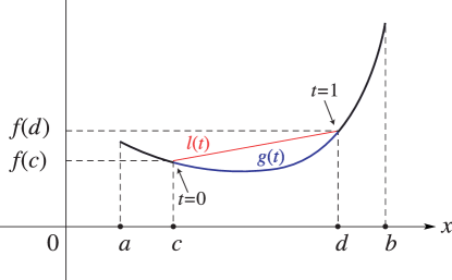
§1.4(vi) Taylor’s Theorem for Real Variables

… ►

►►

Figure 1.4.2: Convex function $f(x)$. … Magnify

5: 18.38 Mathematical Applications

… ►

Quadrature “Extended” to Pseudo-Spectral (DVR) Representations of Operators in One and Many Dimensions

… ►This gives also new structures and results in the one-variable case, but the obtained nonsymmetric special functions can now usually be written as a linear combination of two known special functions. ►In the one-variable case the Dunkl operator eigenvalue equation … ►For the one-variable $q$-case see Noumi and Stokman (2004), Koornwinder (2007a, §§3,4), Koornwinder and Bouzeffour (2011, §§4,5) and Terwilliger (2013). …

6: 31.16 Mathematical Applications

… ►By specifying either $\theta$ or $\varphi$ in (31.16.1) and (31.16.2) we obtain expansions in terms of one variable. …

7: 8.27 Approximations

… ►

Luke (1975, §4.3) gives Padé approximation methods, combined with a detailed analysis of the error terms, valid for real and complex variables except on the negative real $z$-axis. See also Temme (1994b, §3).

…

8: 18.22 Hahn Class: Recurrence Relations and Differences

… ►

§18.22(ii) Difference Equations in $x$

…

9: 18.37 Classical OP’s in Two or More Variables

… ►Orthogonal polynomials associated with root systems are certain systems of trigonometric polynomials in several variables, symmetric under a certain finite group (Weyl group), and orthogonal on a torus. In one variable they are essentially ultraspherical, Jacobi, continuous $q$-ultraspherical, or Askey–Wilson polynomials. …

10: 18.36 Miscellaneous Polynomials

… ►These are polynomials in one variable that are orthogonal with respect to a number of different measures. …