normal equations

SearchAdvancedHelp

(0.002 seconds)

11—20 of 74 matching pages

11: 1.17 Integral and Series Representations of the Dirac Delta

… ►In the language of physics and applied mathematics, these equations indicate the normalizations chosen for these non-$L^2$ improper eigenfunctions of the differential operators (with derivatives respect to spatial co-ordinates) which generate them; the normalizations (1.17.12_1) and (1.17.12_2) are explicitly derived in Friedman (1990, Ch. 4), the others follow similarly. …

12: 29.21 Tables

… ►

Arscott and Khabaza (1962) tabulates the coefficients of the polynomials $P$ in Table 29.12.1 (normalized so that the numerically largest coefficient is unity, i.e. monic polynomials), and the corresponding eigenvalues $h$ for $k^2=0.1(.1)0.9$, $n=1(1)30$. Equations from §29.6 can be used to transform to the normalization adopted in this chapter. Precision is 6S.

13: 30.16 Methods of Computation

… ►If ${\lambda }_n^m\left({\gamma }^2\right)$ is known, then we can compute ${\mathrm{𝖯𝗌}}_n^m(x,{\gamma }^2)$ (not normalized) by solving the differential equation (30.2.1) numerically with initial conditions $w(0)=1$, $w^{\prime }(0)=0$ if $n-m$ is even, or $w(0)=0$, $w^{\prime }(0)=1$ if $n-m$ is odd. …

14: 10.74 Methods of Computation

… ►In the case of $J_n\left(x\right)$, the need for initial values can be avoided by application of Olver’s algorithm (§3.6(v)) in conjunction with Equation (10.12.4) used as a normalizing condition, or in the case of noninteger orders, (10.23.15). …

15: 2.11 Remainder Terms; Stokes Phenomenon

… ►For notational convenience assume that the original differential equation (2.7.1) is normalized so that ${\lambda }_2-{\lambda }_1=1$. …

16: 1.18 Linear Second Order Differential Operators and Eigenfunction Expansions

… ►Applying equations (1.18.29) and (1.18.30), the complete set of normalized eigenfunctions being … ►See Friedman (1990, pp. 233–252) for elementary discussions of both equations and the normalization process; and also the references in §1.18(ix). …

17: 14.30 Spherical and Spheroidal Harmonics

… ►In the quantization of angular momentum the spherical harmonics $Y_{l,m}(\theta ,\varphi )$ are normalized solutions of the eigenvalue equations …

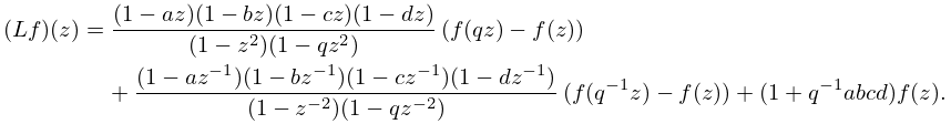
18: 18.28 Askey–Wilson Class

… ►

$q$-Difference Equation

►

18.28.6_1 $$(L{R}_n)(z)=(q^{-n}+abcd{q}^{n-1})R_n(z),$$

ⓘ

Symbols:

$z$: complex variable, $q$: real variable and $n$: nonnegative integer

Referenced by:

§18.28(ii), §18.28(ii), Erratum (V1.2.0) Section 18.28

Permalink:

http://dlmf.nist.gov/18.28.E6_1

Encodings:

pMML, png, TeX

Addition (effective with 1.2.0):

This equation was added.

See also:

Annotations for §18.28(ii), §18.28(ii), §18.28 and Ch.18

… ►

18.28.6_2 $$(Lf)(z)=\frac{(1-az)(1-bz)(1-cz)(1-dz)}{(1-z^2)(1-q{z}^2)}\left(f(qz)-f(z)\right)+\frac{(1-a{z}^{-1})(1-b{z}^{-1})(1-c{z}^{-1})(1-d{z}^{-1})}{(1-z^{-2})(1-q{z}^{-2})}\left(f(q^{-1}z)-f(z)\right)+\left(1+q^{-1}abcd\right)f(z).$$

ⓘ

Symbols:

$z$: complex variable and $q$: real variable

Referenced by:

§18.28(ii), §18.38(iii), §18.38(iii)

Permalink:

http://dlmf.nist.gov/18.28.E6_2

Encodings:

pMML, png, TeX

Addition (effective with 1.2.0):

This equation was added.

See also:

Annotations for §18.28(ii), §18.28(ii), §18.28 and Ch.18

… ►

18.28.6_3 $$(z+z^{-1})R_n(z)=a_n\left(R_{n+1}(z)-R_n(z)\right)+c_n\left(R_{n-1}(z)-R_n(z)\right)+(a+a^{-1})R_n(z),$$

ⓘ

Symbols:

$z$: complex variable and $n$: nonnegative integer

Referenced by:

§18.28(ii)

Permalink:

http://dlmf.nist.gov/18.28.E6_3

Encodings:

pMML, png, TeX

Addition (effective with 1.2.0):

This equation was added.

See also:

Annotations for §18.28(ii), §18.28(ii), §18.28 and Ch.18

… ►

18.28.6_5 $$R_n(a^{-1}{q}^{-m};a,b,c,d|q)=R_m({\tilde{a}}^{-1}{q}^{-n};\tilde{a},\tilde{b},\tilde{c},\tilde{d}|q),$$ $m,n=0,1,2,\mathrm{\dots }$.

ⓘ

Symbols:

$q$: real variable, $m$: nonnegative integer and $n$: nonnegative integer

Referenced by:

§18.28(ii), §18.28(ii), Erratum (V1.2.0) Section 18.28

Permalink:

http://dlmf.nist.gov/18.28.E6_5

Encodings:

pMML, png, TeX

Addition (effective with 1.2.0):

This equation was added.

See also:

Annotations for §18.28(ii), §18.28(ii), §18.28 and Ch.18

…

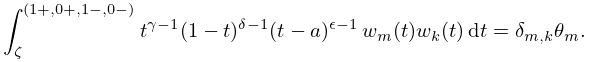
19: 31.9 Orthogonality

… ►

31.9.2 $${\int }_{\zeta }^{(1+,0+,1-,0-)}{t}^{\gamma -1}{(1-t)}^{\delta -1}{(t-a)}^{ϵ-1}{w}_m(t)w_k(t)dt={\delta }_{m,k}{\theta }_m.$$

ⓘ

Symbols:

${\delta }_{j,k}$: Kronecker delta, $dx$: differential of $x$ , $\int$: integral, $\gamma$: real or complex parameter, $\delta$: real or complex parameter, $ϵ$: real or complex parameter, $m$: nonnegative integer, $a$: complex parameter, $\zeta$: point and ${\theta }_m$: normalization constant

Permalink:

http://dlmf.nist.gov/31.9.E2

Encodings:

pMML, png, TeX

See also:

Annotations for §31.9(i), §31.9 and Ch.31

… ►The normalization constant ${\theta }_m$ is given by ►

31.9.3 $${\theta }_m={(1-{\mathrm{e}}^{2\pi \mathrm{i}\gamma })(1-{\mathrm{e}}^{2\pi \mathrm{i}\delta }){\zeta }^{\gamma }{(1-\zeta )}^{\delta }{(\zeta -a)}^{ϵ}\frac{f_0(q,\zeta )}{f_1(q,\zeta )}\frac{\partial }{\partial q}𝒲\left\{f_0(q,\zeta ),f_1(q,\zeta )\right\}|}_{q=q_m},$$

ⓘ

Defines:

${\theta }_m$: normalization constant (locally)

Symbols:

$𝒲$: Wronskian, $\pi$: the ratio of the circumference of a circle to its diameter, $\mathrm{e}$: base of natural logarithm, $\mathrm{i}$: imaginary unit, $\frac{\partial f}{\partial x}$: partial derivative of $f$ with respect to $x$ , $\partial x$: partial differential of $x$ , $\gamma$: real or complex parameter, $\delta$: real or complex parameter, $ϵ$: real or complex parameter, $m$: nonnegative integer, $a$: complex parameter, $q$: real or complex parameter, $\zeta$: point and $f_0(q_m,z)$, $f_1(q_m,z)$: coefficients

Permalink:

http://dlmf.nist.gov/31.9.E3

Encodings:

pMML, png, TeX

See also:

Annotations for §31.9(i), §31.9 and Ch.31

… ►and the integration paths ${ℒ}_1$, ${ℒ}_2$ are Pochhammer double-loop contours encircling distinct pairs of singularities $\{0,1\}$, $\{0,a\}$, $\{1,a\}$. ►For further information, including normalization constants, see Sleeman (1966a). …

20: 8.12 Uniform Asymptotic Expansions for Large Parameter

… ►

8.12.5 $$\frac{{\mathrm{e}}^{\pm \pi \mathrm{i}a}}{2\mathrm{i}\sin \left(\pi a\right)}Q(-a,z{\mathrm{e}}^{\pm \pi \mathrm{i}})=\pm \frac{1}{2}\mathrm{erfc}\left(\pm \mathrm{i}\eta \sqrt{a/2}\right)-\mathrm{i}T(a,\eta ),$$

ⓘ

Symbols:

$\mathrm{\Gamma }\left(z\right)$: gamma function, $\pi$: the ratio of the circumference of a circle to its diameter, $\mathrm{erfc}z$: complementary error function, $\mathrm{e}$: base of natural logarithm, $\mathrm{i}$: imaginary unit, $\mathrm{\Gamma }(a,z)$: incomplete gamma function, $Q(a,z)$: normalized incomplete gamma function, $\sin z$: sine function, $z$: complex variable, $a$: parameter, $\eta (\lambda )$ and $T(a,\eta )$: function

Referenced by:

Erratum (V1.0.16) for Equation (8.12.5), Erratum (V1.0.16) for Equation (8.12.5)

Permalink:

http://dlmf.nist.gov/8.12.E5

Encodings:

pMML, png, TeX

Change (effective with 1.0.16):

To be consistent with the notation used in (8.12.16), the original equation,

$$\mathrm{\Gamma }\left(a+1\right)\frac{{\mathrm{e}}^{\pm \pi \mathrm{i}a}}{2\pi \mathrm{i}}\mathrm{\Gamma }(-a,z{\mathrm{e}}^{\pm \pi \mathrm{i}})=\mp \frac{1}{2}\mathrm{erfc}\left(\pm \mathrm{i}\eta \sqrt{a/2}\right)+\mathrm{i}T(a,\eta ),$$

was rewritten.

See also:

Annotations for §8.12 and Ch.8

… ►

8.12.16 $$\frac{{\mathrm{e}}^{\pm \pi \mathrm{i}a}}{2\mathrm{i}\sin \left(\pi a\right)}Q(-a,a{\mathrm{e}}^{\pm \pi \mathrm{i}})\sim \pm \frac{1}{2}-\frac{\mathrm{i}}{\sqrt{2\pi a}}\sum _{k=0}^{\mathrm{\infty }}{c}_k(0){(-a)}^{-k},$$ $|\mathrm{ph}a|\le \pi -\delta$,

ⓘ

Symbols:

$\sim$: Poincaré asymptotic expansion, $\pi$: the ratio of the circumference of a circle to its diameter, $\mathrm{e}$: base of natural logarithm, $\mathrm{i}$: imaginary unit, $Q(a,z)$: normalized incomplete gamma function, $\mathrm{ph}$: phase, $\sin z$: sine function, $a$: parameter, $k$: nonnegative integer, $\delta$: small positive constant and $c_k(\eta )$: coefficients

Referenced by:

(8.12.5), Erratum (V1.0.16) for Equation (8.12.5)

Permalink:

http://dlmf.nist.gov/8.12.E16

Encodings:

pMML, png, TeX

See also:

Annotations for §8.12 and Ch.8

… ►

8.12.18 $$\begin{array}{c}Q(a,z)\\ P(a,z)\end{array}\}\sim \frac{z^{a-\frac{1}{2}}{\mathrm{e}}^{-z}}{\mathrm{\Gamma }\left(a\right)}\left(d(\pm \chi )\sum _{k=0}^{\mathrm{\infty }}\frac{A_k(\chi )}{z^{k/2}}\mp \sum _{k=1}^{\mathrm{\infty }}\frac{B_k(\chi )}{z^{k/2}}\right),$$

ⓘ

Symbols:

$\mathrm{\Gamma }\left(z\right)$: gamma function, $\sim$: Poincaré asymptotic expansion, $\mathrm{e}$: base of natural logarithm, $P(a,z)$: normalized incomplete gamma function, $Q(a,z)$: normalized incomplete gamma function, $z$: complex variable, $a$: parameter, $k$: nonnegative integer, $\chi$ , $d(\pm \chi )$ , $A_k(\chi )$ and $B_k(\chi )$

Referenced by:

§8.12, Erratum (V1.0.16) for Equation (8.12.18)

Permalink:

http://dlmf.nist.gov/8.12.E18

Encodings:

pMML, png, TeX

Errata (effective with 1.0.16):

The original $\pm$ in front of the second summation was replaced by $\mp$ to correct an error in Paris (2002b); for details see https://arxiv.org/abs/1611.00548.

Reported 2017-01-28 by Richard Paris

See also:

Annotations for §8.12 and Ch.8

…