n-dimensional sphere

(0.003 seconds)

1—10 of 12 matching pages

1: 5.19 Mathematical Applications

… ►

§5.19(iii) $n$ -Dimensional Sphere

►The volume

V

and surface area

S

of the

n

-dimensional sphere of radius

r

are given by …

$x, y$	real variables.
…
$\mathbf{E}_{n}$	the space of all $n$ -dimensional vectors.
…

3: Bibliography R

… ►

M. Robnik (1980) An extremum property of the

n

-dimensional sphere. J. Phys. A 13 (10), pp. L349–L351.

ⓘ

External Links:: ISSN 0305-4470, Document, MathReview
Referenced by:: §5.19(iii).
Encodings:: BibTeX

…

4: 1.2 Elementary Algebra

… ►Let

\left\|{\mathbf{x}}\right\|=\left\|{\mathbf{x}}\right\|_{2}

the

l^{2}

norm, and

\mathbf{E}_{n}

the space of all

n

-dimensional vectors. … ►

1.2.67

\left\|{\mathbf{A}}\right\|=\max_{\mathbf{x}\in\mathbf{E}_{n}\setminus\left\{% \boldsymbol{{0}}\right\}}\frac{\left\|{\mathbf{A}\mathbf{x}}\right\|}{\left\|{% \mathbf{x}}\right\|}=\max_{\left\|{\mathbf{x}}\right\|=1}\left\|{\mathbf{A}% \mathbf{x}}\right\|.

ⓘ

Defines:: $\left\|{\NVar{\mathbf{A}}}\right\|$ : matrix norm
Symbols:: $\in$ : element of, $\setminus$ : set subtraction, $\left\|{\NVar{\mathbf{v}}}\right\|$ : vector norm ( $l$ ²), $\mathbf{E}_{n}$ : space of $n$ -dimensional vectors, real or complex, $\mathbf{A}$ : non-defective matrix and $\boldsymbol{{0}}$ : $m\times m$ matrix of zeros
Permalink:: http://dlmf.nist.gov/1.2.E67
Encodings:: pMML, png, TeX
See also:: Annotations for §1.2(vi), §1.2(vi), §1.2 and Ch.1

…

5: 1.3 Determinants, Linear Operators, and Spectral Expansions

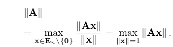
… ►Square matices can be seen as linear operators because

\mathbf{A}(\alpha\mathbf{a}+\beta\mathbf{b})=\alpha\mathbf{A}\mathbf{a}+\beta% \mathbf{A}\mathbf{b}

for all

\alpha,\beta\in\mathbb{C}

and

\mathbf{a},\mathbf{b}\in\mathbf{E}_{n}

, the space of all

n

-dimensional vectors. …

6: 14.31 Other Applications

… ►The conical functions

\mathsf{P}^{m}_{-\frac{1}{2}+i\tau}\left(x\right)

appear in boundary-value problems for the Laplace equation in toroidal coordinates (§14.19(i)) for regions bounded by cones, by two intersecting spheres, or by one or two confocal hyperboloids of revolution (Kölbig (1981)). … ►Many additional physical applications of Legendre polynomials and associated Legendre functions include solution of the Helmholtz equation, as well as the Laplace equation, in spherical coordinates (Temme (1996b)), quantum mechanics (Edmonds (1974)), and high-frequency scattering by a sphere (Nussenzveig (1965)). …

7: 31.17 Physical Applications

… ►Consider the following spectral problem on the sphere

S_{2}

\mathbf{x}^{2}=x_{s}^{2}+x_{t}^{2}+x_{u}^{2}=R^{2}

. …

8: 19.37 Tables

… ►Here

\sigma^{2}=\tfrac{2}{3}((\ln a)^{2}+(\ln b)^{2}+(\ln c)^{2})

\cos\left(3\gamma\right)=(4/\sigma^{3})(\ln a)(\ln b)(\ln c)

, and

a, b, c

are semiaxes of an ellipsoid with the same volume as the unit sphere. …

9: Bibliography N

… ►

H. M. Nussenzveig (1965) High-frequency scattering by an impenetrable sphere. Ann. Physics 34 (1), pp. 23–95.

ⓘ

External Links:: Document, MathReview (E. Ar)
Referenced by:: §14.31(iii).
Encodings:: BibTeX

…

10: 1.6 Vectors and Vector-Valued Functions

… ►For a sphere

x=\rho\sin\theta\cos\phi

y=\rho\sin\theta\sin\phi

z=\rho\cos\theta

, ►

1.6.50

\left\|{\mathbf{T}_{\theta}\times\mathbf{T}_{\phi}}\right\|=\rho^{2}\left|\sin% \theta\right|.

ⓘ

Symbols:: $\sin\NVar{z}$ : sine function, $\left\|{\NVar{\mathbf{v}}}\right\|$ : vector norm ( $l$ ²), $\rho$ : radius, $\theta$ : angle, $\phi$ : angle and $\left|\NVar{x}\right|$ : absolute value of $\NVar{x}$
Permalink:: http://dlmf.nist.gov/1.6.E50
Encodings:: pMML, png, TeX
See also:: Annotations for §1.6(v), §1.6 and Ch.1

…