multivariate hypergeometric function

(0.003 seconds)

1—10 of 25 matching pages

1: 19.15 Advantages of Symmetry

… ►Elliptic integrals are special cases of a particular multivariate hypergeometric function called Lauricella’s

F_{D}

(Carlson (1961b)). …

2: 19.16 Definitions

… ►

§19.16(ii) $R_{-a}\left(\mathbf{b};\mathbf{z}\right)$

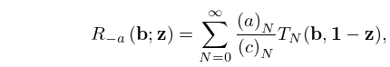
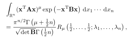
►All elliptic integrals of the form (19.2.3) and many multiple integrals, including (19.23.6) and (19.23.6_5), are special cases of a multivariate hypergeometric function ►

19.16.8

R_{-a}\left(\mathbf{b};\mathbf{z}\right)=R_{-a}\left(b_{1},\dots,b_{n};z_{1},% \dots,z_{n}\right),

ⓘ

Symbols:: $R_{\NVar{-a}}\left(\NVar{b_{1}},\dots,\NVar{b_{n}};\NVar{z_{1}},\dots,\NVar{z_% {n}}\right)$ or $R_{\NVar{-a}}\left(\NVar{\mathbf{b}};\NVar{\mathbf{z}}\right)$ : multivariate hypergeometric function and $n$ : nonnegative integer
Referenced by:: §19.16(ii)
Permalink:: http://dlmf.nist.gov/19.16.E8
Encodings:: pMML, png, TeX
See also:: Annotations for §19.16(ii), §19.16 and Ch.19

… ► … ►

19.16.14

R_{F}\left(x,y,z\right)=R_{-\frac{1}{2}}\left(\tfrac{1}{2},\tfrac{1}{2},\tfrac% {1}{2};x,y,z\right),

ⓘ

Symbols:: $R_{\NVar{-a}}\left(\NVar{b_{1}},\dots,\NVar{b_{n}};\NVar{z_{1}},\dots,\NVar{z_% {n}}\right)$ or $R_{\NVar{-a}}\left(\NVar{\mathbf{b}};\NVar{\mathbf{z}}\right)$ : multivariate hypergeometric function and $R_{F}\left(\NVar{x},\NVar{y},\NVar{z}\right)$ : symmetric elliptic integral of first kind
Referenced by:: §19.16(iii), §19.18(i), §19.18(ii), §19.19, §19.19, §19.24(ii)
Permalink:: http://dlmf.nist.gov/19.16.E14
Encodings:: pMML, png, TeX
See also:: Annotations for §19.16(iii), §19.16 and Ch.19

…

3: Bille C. Carlson

… ►In his paper Lauricella’s hypergeometric function

F_{D}

(1963), he defined the

R

-function, a multivariate hypergeometric function that is homogeneous in its variables, each variable being paired with a parameter. …

4: 19.19 Taylor and Related Series

… ►

19.19.2

R_{-a}\left(\mathbf{b};\mathbf{z}\right)=\sum_{N=0}^{\infty}\frac{{\left(a% \right)_{N}}}{{\left(c\right)_{N}}}T_{N}(\mathbf{b},\boldsymbol{{1}}-\mathbf{z% }),

c=\sum_{j=1}^{n}b_{j}

|1-z_{j}|<1

ⓘ

Symbols:: $R_{\NVar{-a}}\left(\NVar{b_{1}},\dots,\NVar{b_{n}};\NVar{z_{1}},\dots,\NVar{z_% {n}}\right)$ or $R_{\NVar{-a}}\left(\NVar{\mathbf{b}};\NVar{\mathbf{z}}\right)$ : multivariate hypergeometric function, ${\left(\NVar{a}\right)_{\NVar{n}}}$ : Pochhammer’s symbol (or shifted factorial), $n$ : nonnegative integer, $N$ : nonnegative integer and $T_{N}(\mathbf{b},\mathbf{z})$ : polynomial
Referenced by:: §19.19
Permalink:: http://dlmf.nist.gov/19.19.E2
Encodings:: pMML, png, TeX
See also:: Annotations for §19.19 and Ch.19

►

19.19.3

R_{-a}\left(\mathbf{b};\mathbf{z}\right)=z_{n}^{-a}\sum_{N=0}^{\infty}\frac{{% \left(a\right)_{N}}}{{\left(c\right)_{N}}}\*{T_{N}(b_{1},\dots,b_{n-1};1-(z_{1% }/z_{n}),\dots,1-(z_{n-1}/z_{n}))},

c=\sum_{j=1}^{n}b_{j}

|1-(z_{j}/z_{n})|<1

ⓘ

Symbols:: $R_{\NVar{-a}}\left(\NVar{b_{1}},\dots,\NVar{b_{n}};\NVar{z_{1}},\dots,\NVar{z_% {n}}\right)$ or $R_{\NVar{-a}}\left(\NVar{\mathbf{b}};\NVar{\mathbf{z}}\right)$ : multivariate hypergeometric function, ${\left(\NVar{a}\right)_{\NVar{n}}}$ : Pochhammer’s symbol (or shifted factorial), $n$ : nonnegative integer, $N$ : nonnegative integer and $T_{N}(\mathbf{b},\mathbf{z})$ : polynomial
Referenced by:: §19.19, §19.19, §19.28
Permalink:: http://dlmf.nist.gov/19.19.E3
Encodings:: pMML, png, TeX
See also:: Annotations for §19.19 and Ch.19

… ►

19.19.6

R_{J}\left(x,y,z,p\right)=R_{-\frac{3}{2}}\left(\tfrac{1}{2},\tfrac{1}{2},% \tfrac{1}{2},\tfrac{1}{2},\tfrac{1}{2};x,y,z,p,p\right)

ⓘ

Symbols:: $R_{\NVar{-a}}\left(\NVar{b_{1}},\dots,\NVar{b_{n}};\NVar{z_{1}},\dots,\NVar{z_% {n}}\right)$ or $R_{\NVar{-a}}\left(\NVar{\mathbf{b}};\NVar{\mathbf{z}}\right)$ : multivariate hypergeometric function and $R_{J}\left(\NVar{x},\NVar{y},\NVar{z},\NVar{p}\right)$ : symmetric elliptic integral of third kind
Referenced by:: §19.19
Permalink:: http://dlmf.nist.gov/19.19.E6
Encodings:: pMML, png, TeX
See also:: Annotations for §19.19 and Ch.19

… ►

19.19.7

R_{-a}\left(\boldsymbol{{\tfrac{1}{2}}};\mathbf{z}\right)=A^{-a}\sum_{N=0}^{% \infty}\frac{{\left(a\right)_{N}}}{{\left(\tfrac{1}{2}n\right)_{N}}}T_{N}(% \boldsymbol{{\tfrac{1}{2}}},\mathbf{Z}),

ⓘ

Symbols:: $R_{\NVar{-a}}\left(\NVar{b_{1}},\dots,\NVar{b_{n}};\NVar{z_{1}},\dots,\NVar{z_% {n}}\right)$ or $R_{\NVar{-a}}\left(\NVar{\mathbf{b}};\NVar{\mathbf{z}}\right)$ : multivariate hypergeometric function, ${\left(\NVar{a}\right)_{\NVar{n}}}$ : Pochhammer’s symbol (or shifted factorial), $n$ : nonnegative integer, $N$ : nonnegative integer, $T_{N}(\mathbf{b},\mathbf{z})$ : polynomial, $\mathbf{Z}$ : variable and $A$
Referenced by:: §19.15, §19.36(i), §19.36(i), §19.36(i)
Permalink:: http://dlmf.nist.gov/19.19.E7
Encodings:: pMML, png, TeX
See also:: Annotations for §19.19 and Ch.19

…

5: 35.1 Special Notation

… ► ►►

$a, b$	complex variables.
…

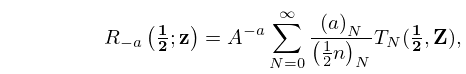
►The main functions treated in this chapter are the multivariate gamma and beta functions, respectively

\Gamma_{m}\left(a\right)

and

\mathrm{B}_{m}\left(a,b\right)

, and the special functions of matrix argument: Bessel (of the first kind)

A_{\nu}\left(\mathbf{T}\right)

and (of the second kind)

B_{\nu}\left(\mathbf{T}\right)

; confluent hypergeometric (of the first kind)

{{}_{1}F_{1}}\left(a;b;\mathbf{T}\right)

\displaystyle{{}_{1}F_{1}}\left({a\atop b};\mathbf{T}\right)

and (of the second kind)

\Psi\left(a;b;\mathbf{T}\right)

; Gaussian hypergeometric

{{}_{2}F_{1}}\left(a_{1},a_{2};b;\mathbf{T}\right)

\displaystyle{{}_{2}F_{1}}\left({a_{1},a_{2}\atop b};\mathbf{T}\right)

; generalized hypergeometric

{{}_{p}F_{q}}\left(a_{1},\dots,a_{p};b_{1},\dots,b_{q};\mathbf{T}\right)

\displaystyle{{}_{p}F_{q}}\left({a_{1},\dots,a_{p}\atop b_{1},\dots,b_{q}};% \mathbf{T}\right)

. … ►Related notations for the Bessel functions are

\mathcal{J}_{\nu+\frac{1}{2}(m+1)}(\mathbf{T})=A_{\nu}\left(\mathbf{T}\right)/% A_{\nu}\left(\boldsymbol{{0}}\right)

(Faraut and Korányi (1994, pp. 320–329)),

K_{m}(0,\dots,0,\nu\mathpunct{|}\mathbf{S},\mathbf{T})=\left|\mathbf{T}\right|% ^{\nu}B_{\nu}\left(\mathbf{S}\mathbf{T}\right)

(Terras (1988, pp. 49–64)), and

\mathcal{K}_{\nu}(\mathbf{T})=\left|\mathbf{T}\right|^{\nu}B_{\nu}\left(% \mathbf{S}\mathbf{T}\right)

(Faraut and Korányi (1994, pp. 357–358)).

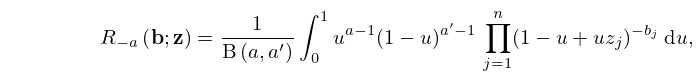
6: 19.31 Probability Distributions

… ►

19.31.2

\int_{{\mathbb{R}}^{n}}(\mathbf{x}^{\mathrm{T}}\mathbf{A}\mathbf{x})^{\mu}\exp% \left(-\mathbf{x}^{\mathrm{T}}\mathbf{B}\mathbf{x}\right)\,\mathrm{d}x_{1}% \cdots\,\mathrm{d}x_{n}=\frac{\pi^{n/2}\Gamma\left(\mu+\tfrac{1}{2}n\right)}{% \sqrt{\det\mathbf{B}}\Gamma\left(\tfrac{1}{2}n\right)}R_{\mu}\left(\tfrac{1}{2% },\dots,\tfrac{1}{2};\lambda_{1},\dots,\lambda_{n}\right),

\mu>-\tfrac{1}{2}n

ⓘ

Symbols:: $R_{\NVar{-a}}\left(\NVar{b_{1}},\dots,\NVar{b_{n}};\NVar{z_{1}},\dots,\NVar{z_% {n}}\right)$ or $R_{\NVar{-a}}\left(\NVar{\mathbf{b}};\NVar{\mathbf{z}}\right)$ : multivariate hypergeometric function, $\Gamma\left(\NVar{z}\right)$ : gamma function, $\pi$ : the ratio of the circumference of a circle to its diameter, $\det$ : determinant, $\,\mathrm{d}\NVar{x}$ : differential of $x$ , $\exp\NVar{z}$ : exponential function, $\int$ : integral, $\mathbb{R}$ : real line, $\NVar{\mathbf{A}}^{\mathrm{T}}$ : transpose of matrix, $n$ : nonnegative integer and $\lambda_{n}$ : eigenvalues
Referenced by:: §19.31
Permalink:: http://dlmf.nist.gov/19.31.E2
Encodings:: pMML, png, TeX
See also:: Annotations for §19.31 and Ch.19

…

7: 19.1 Special Notation

… ►

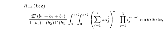
R_{-a}\left(b_{1},b_{2},\dots,b_{n};z_{1},z_{2},\dots,z_{n}\right)

is a multivariate hypergeometric function that includes all the functions in (19.1.3). …

8: 19.23 Integral Representations

… ►

19.23.8

R_{-a}\left(\mathbf{b};\mathbf{z}\right)=\frac{2}{\mathrm{B}\left(b_{1},b_{2}% \right)}\int_{0}^{\pi/2}{(z_{1}{\cos}^{2}\theta+z_{2}{\sin}^{2}\theta)}^{-a}\*% (\cos\theta)^{2b_{1}-1}(\sin\theta)^{2b_{2}-1}\,\mathrm{d}\theta,

b_{1},b_{2}>0

;

\Re z_{1},\Re z_{2}>0

ⓘ

Symbols:: $R_{\NVar{-a}}\left(\NVar{b_{1}},\dots,\NVar{b_{n}};\NVar{z_{1}},\dots,\NVar{z_% {n}}\right)$ or $R_{\NVar{-a}}\left(\NVar{\mathbf{b}};\NVar{\mathbf{z}}\right)$ : multivariate hypergeometric function, $\mathrm{B}\left(\NVar{a},\NVar{b}\right)$ : beta function, $\pi$ : the ratio of the circumference of a circle to its diameter, $\cos\NVar{z}$ : cosine function, $\,\mathrm{d}\NVar{x}$ : differential of $x$ , $\int$ : integral, $\Re$ : real part and $\sin\NVar{z}$ : sine function
Referenced by:: §19.2(iv), §19.23, §19.23, §19.23
Permalink:: http://dlmf.nist.gov/19.23.E8
Encodings:: pMML, png, TeX
See also:: Annotations for §19.23 and Ch.19

… ►

19.23.9

R_{-a}\left(\mathbf{b};\mathbf{z}\right)=\frac{4\Gamma\left(b_{1}+b_{2}+b_{3}% \right)}{\Gamma\left(b_{1}\right)\Gamma\left(b_{2}\right)\Gamma\left(b_{3}% \right)}\int_{0}^{\pi/2}\!\!\!\!\int_{0}^{\pi/2}\left(\sum_{j=1}^{3}z_{j}l_{j}% ^{2}\right)^{-a}\*\prod_{j=1}^{3}l_{j}^{2b_{j}-1}\sin\theta\,\mathrm{d}\theta% \,\mathrm{d}\phi,

b_{j}>0

\Re z_{j}>0

ⓘ

Symbols:: $R_{\NVar{-a}}\left(\NVar{b_{1}},\dots,\NVar{b_{n}};\NVar{z_{1}},\dots,\NVar{z_% {n}}\right)$ or $R_{\NVar{-a}}\left(\NVar{\mathbf{b}};\NVar{\mathbf{z}}\right)$ : multivariate hypergeometric function, $\Gamma\left(\NVar{z}\right)$ : gamma function, $\pi$ : the ratio of the circumference of a circle to its diameter, $\,\mathrm{d}\NVar{x}$ : differential of $x$ , $\int$ : integral, $\Re$ : real part, $\sin\NVar{z}$ : sine function, $l$ : nonnegative integer and $\phi$ : real or complex argument
Referenced by:: §19.23, §19.23
Permalink:: http://dlmf.nist.gov/19.23.E9
Encodings:: pMML, png, TeX
See also:: Annotations for §19.23 and Ch.19

►

19.23.10

R_{-a}\left(\mathbf{b};\mathbf{z}\right)=\frac{1}{\mathrm{B}\left(a,a^{\prime}% \right)}\int_{0}^{1}u^{a-1}(1-u)^{a^{\prime}-1}\*\prod_{j=1}^{n}(1-u+uz_{j})^{% -b_{j}}\,\mathrm{d}u,

a,a^{\prime}>0

;

a+a^{\prime}=\sum_{j=1}^{n}b_{j}

;

z_{j}\in\mathbb{C}\setminus(-\infty,0]

ⓘ

Symbols:: $R_{\NVar{-a}}\left(\NVar{b_{1}},\dots,\NVar{b_{n}};\NVar{z_{1}},\dots,\NVar{z_% {n}}\right)$ or $R_{\NVar{-a}}\left(\NVar{\mathbf{b}};\NVar{\mathbf{z}}\right)$ : multivariate hypergeometric function, $\mathrm{B}\left(\NVar{a},\NVar{b}\right)$ : beta function, $\mathbb{C}$ : complex plane, $\,\mathrm{d}\NVar{x}$ : differential of $x$ , $\in$ : element of, $\int$ : integral, $(\NVar{a},\NVar{b}]$ : half-closed interval, $\setminus$ : set subtraction and $n$ : nonnegative integer
Referenced by:: §19.19, §19.23, §19.23
Permalink:: http://dlmf.nist.gov/19.23.E10
Encodings:: pMML, png, TeX
See also:: Annotations for §19.23 and Ch.19

…

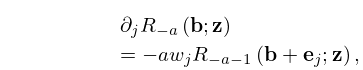
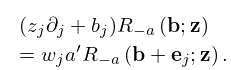
9: 19.18 Derivatives and Differential Equations

… ►

19.18.4

\partial_{j}R_{-a}\left(\mathbf{b};\mathbf{z}\right)=-aw_{j}R_{-a-1}\left(% \mathbf{b}+\mathbf{e}_{j};\mathbf{z}\right),

ⓘ

Symbols:: $R_{\NVar{-a}}\left(\NVar{b_{1}},\dots,\NVar{b_{n}};\NVar{z_{1}},\dots,\NVar{z_% {n}}\right)$ or $R_{\NVar{-a}}\left(\NVar{\mathbf{b}};\NVar{\mathbf{z}}\right)$ : multivariate hypergeometric function, $\,\partial\NVar{x}$ : partial differential of $x$ and $w_{j}$
Referenced by:: §19.18(i), §19.25(i)
Permalink:: http://dlmf.nist.gov/19.18.E4
Encodings:: pMML, png, TeX
See also:: Annotations for §19.18(i), §19.18 and Ch.19

►

19.18.5

(z_{j}\partial_{j}+b_{j})R_{-a}\left(\mathbf{b};\mathbf{z}\right)=w_{j}a^{% \prime}R_{-a}\left(\mathbf{b}+\mathbf{e}_{j};\mathbf{z}\right).

ⓘ

Symbols:: $R_{\NVar{-a}}\left(\NVar{b_{1}},\dots,\NVar{b_{n}};\NVar{z_{1}},\dots,\NVar{z_% {n}}\right)$ or $R_{\NVar{-a}}\left(\NVar{\mathbf{b}};\NVar{\mathbf{z}}\right)$ : multivariate hypergeometric function, $\,\partial\NVar{x}$ : partial differential of $x$ and $w_{j}$
Referenced by:: §19.18(i)
Permalink:: http://dlmf.nist.gov/19.18.E5
Encodings:: pMML, png, TeX
See also:: Annotations for §19.18(i), §19.18 and Ch.19

… ►

19.18.8

\sum_{j=1}^{n}\partial_{j}R_{-a}\left(\mathbf{b};\mathbf{z}\right)=-aR_{-a-1}% \left(\mathbf{b};\mathbf{z}\right).

ⓘ

Symbols:: $R_{\NVar{-a}}\left(\NVar{b_{1}},\dots,\NVar{b_{n}};\NVar{z_{1}},\dots,\NVar{z_% {n}}\right)$ or $R_{\NVar{-a}}\left(\NVar{\mathbf{b}};\NVar{\mathbf{z}}\right)$ : multivariate hypergeometric function, $\,\partial\NVar{x}$ : partial differential of $x$ and $n$ : nonnegative integer
Referenced by:: §19.18(i), §19.18(ii)
Permalink:: http://dlmf.nist.gov/19.18.E8
Encodings:: pMML, png, TeX
See also:: Annotations for §19.18(ii), §19.18 and Ch.19

…

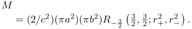
10: 19.34 Mutual Inductance of Coaxial Circles

… ►

19.34.7

M=(2/{c}^{2})(\pi a^{2})(\pi b^{2})R_{-\frac{3}{2}}\left(\tfrac{3}{2},\tfrac{3% }{2};r_{+}^{2},r_{-}^{2}\right).

ⓘ

Symbols:: $R_{\NVar{-a}}\left(\NVar{b_{1}},\dots,\NVar{b_{n}};\NVar{z_{1}},\dots,\NVar{z_% {n}}\right)$ or $R_{\NVar{-a}}\left(\NVar{\mathbf{b}};\NVar{\mathbf{z}}\right)$ : multivariate hypergeometric function, $\pi$ : the ratio of the circumference of a circle to its diameter, $M$ : mutual inductance and $r_{\pm}$
Referenced by:: §19.34
Permalink:: http://dlmf.nist.gov/19.34.E7
Encodings:: pMML, png, TeX
See also:: Annotations for §19.34 and Ch.19

…