modulus

SearchAdvancedHelp

(0.001 seconds)

11—20 of 532 matching pages

11: 22.5 Special Values

… ►For example, at $z=K+\mathrm{i}{K}^{\prime }$, $\mathrm{sn}(z,k)=1/k$, $d\mathrm{sn}(z,k)/dz=0$. (The modulus $k$ is suppressed throughout the table.) … ►For example, $\mathrm{sn}(\frac{1}{2}K,k)={(1+k^{\prime })}^{-1/2}$. … ►

§22.5(ii) Limiting Values of $k$

… ►For values of $K,K^{\prime }$ when $k^2=\frac{1}{2}$ (lemniscatic case) see §23.5(iii), and for $k^2={\mathrm{e}}^{\mathrm{i}\pi /3}$ (equianharmonic case) see §23.5(v). …

12: 36.3 Visualizations of Canonical Integrals

… ►

§36.3(i) Canonical Integrals: Modulus

►

…

Figure 36.3.1: Modulus of Pearcey integral $|{\mathrm{\Psi }}_2\left(x,y\right)|$.

►

…

Figure 36.3.2: Modulus of swallowtail canonical integral function $|{\mathrm{\Psi }}_3\left(x,y,3\right)|$.

►

…

Figure 36.3.3: Modulus of swallowtail canonical integral function $|{\mathrm{\Psi }}_3\left(x,y,0\right)|$.

… ►

…

Figure 36.3.12: Modulus of hyperbolic umbilic canonical integral function $|{\mathrm{\Psi }}^{(\mathrm{H})}\left(x,y,3\right)|$. …

…

13: 4.16 Elementary Properties

… ►

Table 4.16.3: Trigonometric functions: interrelations. …

► ►►►►►►►

	$\sin \theta =a$	$\cos \theta =a$	$\tan \theta =a$	$\csc \theta =a$	$\sec \theta =a$	$\cot \theta =a$
$\sin \theta$	$a$	${(1-a^2)}^{1/2}$	$a{(1+a^2)}^{-1/2}$	$a^{-1}$	$a^{-1}{(a^2-1)}^{1/2}$	${(1+a^2)}^{-1/2}$
$\cos \theta$	${(1-a^2)}^{1/2}$	$a$	${(1+a^2)}^{-1/2}$	$a^{-1}{(a^2-1)}^{1/2}$	$a^{-1}$	$a{(1+a^2)}^{-1/2}$
$\tan \theta$	$a{(1-a^2)}^{-1/2}$	$a^{-1}{(1-a^2)}^{1/2}$	$a$	${(a^2-1)}^{-1/2}$	${(a^2-1)}^{1/2}$	$a^{-1}$
$\csc \theta$	$a^{-1}$	${(1-a^2)}^{-1/2}$	$a^{-1}{(1+a^2)}^{1/2}$	$a$	$a{(a^2-1)}^{-1/2}$	${(1+a^2)}^{1/2}$
$\sec \theta$	${(1-a^2)}^{-1/2}$	$a^{-1}$	${(1+a^2)}^{1/2}$	$a{(a^2-1)}^{-1/2}$	$a$	$a^{-1}{(1+a^2)}^{1/2}$
…

►

14: 10.18 Modulus and Phase Functions

§10.18 Modulus and Phase Functions

►

§10.18(i) Definitions

… ►where $M_{\nu }\left(x\right)$ $(>0)$, $N_{\nu }\left(x\right)$ $(>0)$, ${\theta }_{\nu }\left(x\right)$, and ${\varphi }_{\nu }\left(x\right)$ are continuous real functions of $\nu$ and $x$, with the branches of ${\theta }_{\nu }\left(x\right)$ and ${\varphi }_{\nu }\left(x\right)$ fixed by … ►

§10.18(ii) Basic Properties

… ►

§10.18(iii) Asymptotic Expansions for Large Argument

…

15: 10.55 Continued Fractions

… ►For continued fractions for ${𝗃}_{n+1}\left(z\right)/{𝗃}_n\left(z\right)$ and ${𝗂}_{n+1}^{(1)}\left(z\right)/{𝗂}_n^{(1)}\left(z\right)$ see Cuyt et al. (2008, pp. 350, 353, 362, 363, 367–369).

16: 12.6 Continued Fraction

… ►For a continued-fraction expansion of the ratio $U(a,x)/U(a-1,x)$ see Cuyt et al. (2008, pp. 340–341).

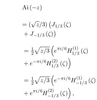
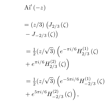
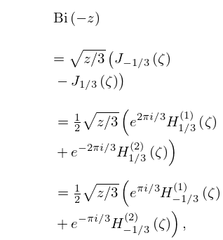
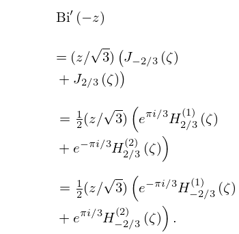
17: 9.6 Relations to Other Functions

… ►

9.6.3 $${\mathrm{Ai}}^{\prime }\left(z\right)=-{\pi }^{-1}(z/\sqrt{3})K_{\pm 2/3}\left(\zeta \right)=(z/3)\left(I_{2/3}\left(\zeta \right)-I_{-2/3}\left(\zeta \right)\right)=\frac{1}{2}(z/\sqrt{3}){\mathrm{e}}^{-\pi \mathrm{i}/6}{H}_{2/3}^{(1)}\left(\zeta {\mathrm{e}}^{\pi \mathrm{i}/2}\right)=\frac{1}{2}(z/\sqrt{3}){\mathrm{e}}^{-5\pi \mathrm{i}/6}{H}_{-2/3}^{(1)}\left(\zeta {\mathrm{e}}^{\pi \mathrm{i}/2}\right)=\frac{1}{2}(z/\sqrt{3}){\mathrm{e}}^{\pi \mathrm{i}/6}{H}_{2/3}^{(2)}\left(\zeta {\mathrm{e}}^{-\pi \mathrm{i}/2}\right)=\frac{1}{2}(z/\sqrt{3}){\mathrm{e}}^{5\pi \mathrm{i}/6}{H}_{-2/3}^{(2)}\left(\zeta {\mathrm{e}}^{-\pi \mathrm{i}/2}\right),$$

ⓘ

Symbols:

$\mathrm{Ai}\left(z\right)$: Airy function, $H_{\nu }^{(1)}\left(z\right)$: Bessel function of the third kind (or Hankel function), $H_{\nu }^{(2)}\left(z\right)$: Bessel function of the third kind (or Hankel function), $\pi$: the ratio of the circumference of a circle to its diameter, $\mathrm{e}$: base of natural logarithm, $\mathrm{i}$: imaginary unit, $I_{\nu }\left(z\right)$: modified Bessel function of the first kind, $K_{\nu }\left(z\right)$: modified Bessel function of the second kind, $z$: complex variable and $\zeta$: change of variable

Proof sketch:

Derivable from those given in Miller (1946, p. B17) and Olver (1997b, pp. 392–393).

A&S Ref:

10.4.16 (with opposite sign!)

Referenced by:

(9.6.22)

Permalink:

http://dlmf.nist.gov/9.6.E3

Encodings:

pMML, png, TeX

See also:

Annotations for §9.6(i), §9.6 and Ch.9

… ►

9.6.6 $$\mathrm{Ai}\left(-z\right)=(\sqrt{z}/3)\left(J_{1/3}\left(\zeta \right)+J_{-1/3}\left(\zeta \right)\right)=\frac{1}{2}\sqrt{z/3}\left({\mathrm{e}}^{\pi \mathrm{i}/6}{H}_{1/3}^{(1)}\left(\zeta \right)+{\mathrm{e}}^{-\pi \mathrm{i}/6}{H}_{1/3}^{(2)}\left(\zeta \right)\right)=\frac{1}{2}\sqrt{z/3}\left({\mathrm{e}}^{-\pi \mathrm{i}/6}{H}_{-1/3}^{(1)}\left(\zeta \right)+{\mathrm{e}}^{\pi \mathrm{i}/6}{H}_{-1/3}^{(2)}\left(\zeta \right)\right),$$

ⓘ

Symbols:

$\mathrm{Ai}\left(z\right)$: Airy function, $J_{\nu }\left(z\right)$: Bessel function of the first kind, $H_{\nu }^{(1)}\left(z\right)$: Bessel function of the third kind (or Hankel function), $H_{\nu }^{(2)}\left(z\right)$: Bessel function of the third kind (or Hankel function), $\pi$: the ratio of the circumference of a circle to its diameter, $\mathrm{e}$: base of natural logarithm, $\mathrm{i}$: imaginary unit, $z$: complex variable and $\zeta$: change of variable

Proof sketch:

Derivable from those given in Miller (1946, p. B17) and Olver (1997b, pp. 392–393).

A&S Ref:

10.4.15 (partial)

Permalink:

http://dlmf.nist.gov/9.6.E6

Encodings:

pMML, png, TeX

See also:

Annotations for §9.6(i), §9.6 and Ch.9

►

9.6.7 $${\mathrm{Ai}}^{\prime }\left(-z\right)=(z/3)\left(J_{2/3}\left(\zeta \right)-J_{-2/3}\left(\zeta \right)\right)=\frac{1}{2}(z/\sqrt{3})\left({\mathrm{e}}^{-\pi \mathrm{i}/6}{H}_{2/3}^{(1)}\left(\zeta \right)+{\mathrm{e}}^{\pi \mathrm{i}/6}{H}_{2/3}^{(2)}\left(\zeta \right)\right)=\frac{1}{2}(z/\sqrt{3})\left({\mathrm{e}}^{-5\pi \mathrm{i}/6}{H}_{-2/3}^{(1)}\left(\zeta \right)+{\mathrm{e}}^{5\pi \mathrm{i}/6}{H}_{-2/3}^{(2)}\left(\zeta \right)\right),$$

ⓘ

Symbols:

$\mathrm{Ai}\left(z\right)$: Airy function, $J_{\nu }\left(z\right)$: Bessel function of the first kind, $H_{\nu }^{(1)}\left(z\right)$: Bessel function of the third kind (or Hankel function), $H_{\nu }^{(2)}\left(z\right)$: Bessel function of the third kind (or Hankel function), $\pi$: the ratio of the circumference of a circle to its diameter, $\mathrm{e}$: base of natural logarithm, $\mathrm{i}$: imaginary unit, $z$: complex variable and $\zeta$: change of variable

Proof sketch:

Derivable from those given in Miller (1946, p. B17) and Olver (1997b, pp. 392–393).

A&S Ref:

10.4.17 (partial)

Permalink:

http://dlmf.nist.gov/9.6.E7

Encodings:

pMML, png, TeX

See also:

Annotations for §9.6(i), §9.6 and Ch.9

►

9.6.8 $$\mathrm{Bi}\left(-z\right)=\sqrt{z/3}\left(J_{-1/3}\left(\zeta \right)-J_{1/3}\left(\zeta \right)\right)=\frac{1}{2}\sqrt{z/3}\left({\mathrm{e}}^{2\pi \mathrm{i}/3}{H}_{1/3}^{(1)}\left(\zeta \right)+{\mathrm{e}}^{-2\pi \mathrm{i}/3}{H}_{1/3}^{(2)}\left(\zeta \right)\right)=\frac{1}{2}\sqrt{z/3}\left({\mathrm{e}}^{\pi \mathrm{i}/3}{H}_{-1/3}^{(1)}\left(\zeta \right)+{\mathrm{e}}^{-\pi \mathrm{i}/3}{H}_{-1/3}^{(2)}\left(\zeta \right)\right),$$

ⓘ

Symbols:

$\mathrm{Bi}\left(z\right)$: Airy function, $J_{\nu }\left(z\right)$: Bessel function of the first kind, $H_{\nu }^{(1)}\left(z\right)$: Bessel function of the third kind (or Hankel function), $H_{\nu }^{(2)}\left(z\right)$: Bessel function of the third kind (or Hankel function), $\pi$: the ratio of the circumference of a circle to its diameter, $\mathrm{e}$: base of natural logarithm, $\mathrm{i}$: imaginary unit, $z$: complex variable and $\zeta$: change of variable

Proof sketch:

Derivable from those given in Miller (1946, p. B17) and Olver (1997b, pp. 392–393).

A&S Ref:

10.4.19 (in slightly different form)

Permalink:

http://dlmf.nist.gov/9.6.E8

Encodings:

pMML, png, TeX

See also:

Annotations for §9.6(i), §9.6 and Ch.9

►

9.6.9 $${\mathrm{Bi}}^{\prime }\left(-z\right)=(z/\sqrt{3})\left(J_{-2/3}\left(\zeta \right)+J_{2/3}\left(\zeta \right)\right)=\frac{1}{2}(z/\sqrt{3})\left({\mathrm{e}}^{\pi \mathrm{i}/3}{H}_{2/3}^{(1)}\left(\zeta \right)+{\mathrm{e}}^{-\pi \mathrm{i}/3}{H}_{2/3}^{(2)}\left(\zeta \right)\right)=\frac{1}{2}(z/\sqrt{3})\left({\mathrm{e}}^{-\pi \mathrm{i}/3}{H}_{-2/3}^{(1)}\left(\zeta \right)+{\mathrm{e}}^{\pi \mathrm{i}/3}{H}_{-2/3}^{(2)}\left(\zeta \right)\right).$$

ⓘ

Symbols:

$\mathrm{Bi}\left(z\right)$: Airy function, $J_{\nu }\left(z\right)$: Bessel function of the first kind, $H_{\nu }^{(1)}\left(z\right)$: Bessel function of the third kind (or Hankel function), $H_{\nu }^{(2)}\left(z\right)$: Bessel function of the third kind (or Hankel function), $\pi$: the ratio of the circumference of a circle to its diameter, $\mathrm{e}$: base of natural logarithm, $\mathrm{i}$: imaginary unit, $z$: complex variable and $\zeta$: change of variable

Proof sketch:

Derivable from those given in Miller (1946, p. B17) and Olver (1997b, pp. 392–393).

A&S Ref:

10.4.21 (partial)

Permalink:

http://dlmf.nist.gov/9.6.E9

Encodings:

pMML, png, TeX

See also:

Annotations for §9.6(i), §9.6 and Ch.9

…

18: 9.3 Graphics

… ►

§9.3(i) Real Variable

►

►►

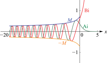
Figure 9.3.1: $\mathrm{Ai}\left(x\right)$, $\mathrm{Bi}\left(x\right)$, $M\left(x\right)$. For $M\left(x\right)$ see §9.8(i). Magnify

►

►►

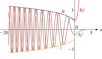
Figure 9.3.2: ${\mathrm{Ai}}^{\prime }\left(x\right)$, ${\mathrm{Bi}}^{\prime }\left(x\right)$, $N\left(x\right)$. For $N\left(x\right)$ see §9.8(i). Magnify

…

19: 11.8 Analogs to Kelvin Functions

§11.8 Analogs to Kelvin Functions

►For properties of Struve functions of argument $x{\mathrm{e}}^{\pm 3\pi \mathrm{i}/4}$ see McLachlan and Meyers (1936).

20: 4.17 Special Values and Limits

… ►

Table 4.17.1: Trigonometric functions: values at multiples of $\frac{1}{12}\pi$.

► ►►►►►►►

$\theta$	$\sin \theta$	$\cos \theta$	$\tan \theta$	$\csc \theta$	$\sec \theta$	$\cot \theta$
…
$\pi /6$	$\frac{1}{2}$	$\frac{1}{2}\sqrt{3}$	$\frac{1}{3}\sqrt{3}$	$2$	$\frac{2}{3}\sqrt{3}$	$\sqrt{3}$
$\pi /4$	$\frac{1}{2}\sqrt{2}$	$\frac{1}{2}\sqrt{2}$	$1$	$\sqrt{2}$	$\sqrt{2}$	$1$
$\pi /3$	$\frac{1}{2}\sqrt{3}$	$\frac{1}{2}$	$\sqrt{3}$	$\frac{2}{3}\sqrt{3}$	$2$	$\frac{1}{3}\sqrt{3}$
…
$\pi /2$	1	0	$\mathrm{\infty }$	1	$\mathrm{\infty }$	0
…
$2\pi /3$	$\frac{1}{2}\sqrt{3}$	$-\frac{1}{2}$	$-\sqrt{3}$	$\frac{2}{3}\sqrt{3}$	$-2$	$-\frac{1}{3}\sqrt{3}$
…

►

…