Zhang and Jin (1996, pp. 638, 640–641) includes the real and imaginary parts
of , , , 7D and 8D, respectively;
the real and imaginary parts of
,
,
, 8D, together with the corresponding modulus and phase to 8D
and 6D (degrees), respectively.
The main tables in Abramowitz and Stegun (1964, Chapter 9) give
to 15D, , ,
, to 10D, to 8D,
; , ,
, 8D; , , ,
, 5D or 5S; , ,
, , 10S; modulus and phase functions
, , ,
, 8D.
Miller (1946) tabulates
, for
,
for ;
, for ;
,
for ; ,
, ,
(respectively , , , ) for .
Precision is generally 8D; slightly less for some of the auxiliary functions.
Extracts from these tables are included in
Abramowitz and Stegun (1964, Chapter 10), together with some auxiliary functions
for large arguments.
…
►As in the sector ,
…
►Wrench (1968) gives exact values of up to .
…
►If is complex, then the remainder terms are bounded in magnitude by for (5.11.1), and for (5.11.2), times the first neglected terms.
…
►For this result and a similar bound for the sector see Boyd (1994).
…
►If in the sector , then
…
…
►For , there are two solutions , provided that .
…
►This consists of three separate cusp-edged sheets connected to the cusp-edged sheets of the bifurcation set, and related by rotation about the -axis by .
…
…
►Then is the circular
frequency of oscillation (with the ordinary frequency), independent of the amplitude of the oscillations.
…With the normalization factor the are orthonormal in .
…
►(where the minus sign is often omitted, as it arises as an arbitrary phase when taking the square root of the real, positive, norm of the wave function), allowing equation (18.39.37) to be rewritten in terms of the associated Coulomb–Laguerre polynomials .
…
►Derivations of (18.39.42) appear in Bethe and Salpeter (1957, pp. 12–20), and Pauling and Wilson (1985, Chapter V and Appendix VII), where the derivations are based on (18.39.36), and is also the notation of Piela (2014, §4.7), typifying the common use of the associated Coulomb–Laguerre polynomials in theoretical quantum chemistry.
…
►For applications and an extension of the Szegő–Szász inequality (18.14.20) for Legendre polynomials () to obtain global bounds on the variation of the phase of an elastic scattering amplitude, see Cornille and Martin (1972, 1974).
…
…
►They lie in the sectors and , and are denoted by , , respectively, in the former sector, and by , , in the conjugate sector, again arranged in ascending order of absolute value (modulus) for See §9.3(ii) for visualizations.
…
►
