modular transformations

(0.002 seconds)

1—10 of 13 matching pages

1: 23.18 Modular Transformations

§23.18 Modular Transformations

… ►

23.18.3

\lambda\left(\mathcal{A}\tau\right)=\lambda\left(\tau\right),

ⓘ

Symbols:: $\lambda\left(\NVar{\tau}\right)$ : elliptic modular function, $\tau$ : complex variable and $\mathcal{A}$ : bilinear transformation
Permalink:: http://dlmf.nist.gov/23.18.E3
Encodings:: pMML, png, TeX
See also:: Annotations for §23.18, §23.18 and Ch.23

… ►

23.18.4

J\left(\mathcal{A}\tau\right)=J\left(\tau\right).

ⓘ

Symbols:: $J\left(\NVar{\tau}\right)$ : Klein’s complete invariant, $\tau$ : complex variable and $\mathcal{A}$ : bilinear transformation
Referenced by:: §23.18
Permalink:: http://dlmf.nist.gov/23.18.E4
Encodings:: pMML, png, TeX
See also:: Annotations for §23.18, §23.18 and Ch.23

… ►

23.18.5

\eta\left(\mathcal{A}\tau\right)=\varepsilon(\mathcal{A})\left(-i(c\tau+d)% \right)^{1/2}\eta\left(\tau\right),

ⓘ

Symbols:: $\eta\left(\NVar{\tau}\right)$ : Dedekind’s eta function (or Dedekind modular function), $\mathrm{i}$ : imaginary unit, $\tau$ : complex variable, $\mathcal{A}$ : bilinear transformation, $c$ : integer, $d$ : integer and $\varepsilon(\mathcal{A})$ : function
Permalink:: http://dlmf.nist.gov/23.18.E5
Encodings:: pMML, png, TeX
See also:: Annotations for §23.18, §23.18 and Ch.23

…

2: 21.5 Modular Transformations

§21.5 Modular Transformations

►

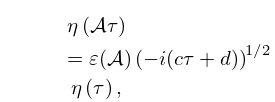
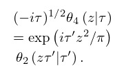
§21.5(i) Riemann Theta Functions

… ►Equation (21.5.4) is the modular transformation property for Riemann theta functions. … ►

§21.5(ii) Riemann Theta Functions with Characteristics

… ►For explicit results in the case

g=1

, see §20.7(viii).

3: 17.18 Methods of Computation

… ►The two main methods for computing basic hypergeometric functions are: (1) numerical summation of the defining series given in §§17.4(i) and 17.4(ii); (2) modular transformations. …

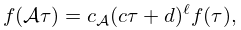
4: 20.7 Identities

… ►

20.7.33

(-i\tau)^{1/2}\theta_{4}\left(z\middle|\tau\right)=\exp\left(i\tau^{\prime}z^{% 2}/\pi\right)\theta_{2}\left(z\tau^{\prime}\middle|\tau^{\prime}\right).

ⓘ

Symbols:: $\theta_{\NVar{j}}\left(\NVar{z}\middle|\NVar{\tau}\right)$ : theta function, $\pi$ : the ratio of the circumference of a circle to its diameter, $\exp\NVar{z}$ : exponential function, $\mathrm{i}$ : imaginary unit, $z$ : complex and $\tau$ : lattice parameter
Referenced by:: (20.10.3), §20.13
Permalink:: http://dlmf.nist.gov/20.7.E33
Encodings:: pMML, png, TeX
See also:: Annotations for §20.7(viii), §20.7 and Ch.20

►These are specific examples of modular transformations as discussed in §23.15; the corresponding results for the general case are given by Rademacher (1973, pp. 181–183). …

5: 23.15 Definitions

… ►

23.15.5

f(\mathcal{A}\tau)=c_{\mathcal{A}}(c\tau+d)^{\ell}f(\tau),

\Im\tau>0

ⓘ

Symbols:: $\Im$ : imaginary part, $\tau$ : complex variable, $\mathcal{A}$ : bilinear transformation, $c$ : integer, $d$ : integer, $f(\tau)$ : modular function, $c_{\mathcal{A}}$ : constant and $\ell$ : level
Permalink:: http://dlmf.nist.gov/23.15.E5
Encodings:: pMML, png, TeX
See also:: Annotations for §23.15(i), §23.15 and Ch.23

…

6: 20.11 Generalizations and Analogs

… ►If both

m, n

are positive, then

G(m,n)

allows inversion of its arguments as a modular transformation (compare (23.15.3) and (23.15.4)): …

7: 27.14 Unrestricted Partitions

… ►Dedekind sums occur in the transformation theory of the Dedekind modular function

\eta\left(\tau\right)

, defined by …

8: Bibliography V

… ►

G. Valent (1986) An integral transform involving Heun functions and a related eigenvalue problem. SIAM J. Math. Anal. 17 (3), pp. 688–703.

ⓘ

External Links:: ISSN 0036-1410, Document, MathReview (William L. Perry), ZentralBlatt
Referenced by:: §31.10(i).
Encodings:: BibTeX

… ►

J. F. Van Diejen and V. P. Spiridonov (2001) Modular hypergeometric residue sums of elliptic Selberg integrals. Lett. Math. Phys. 58 (3), pp. 223–238.

ⓘ

External Links:: ISSN 0377-9017, Document, MathReview (Laurent Habsieger), ZentralBlatt
Referenced by:: §19.35(i).
Encodings:: BibTeX

►

C. Van Loan (1992) Computational Frameworks for the Fast Fourier Transform. Frontiers in Applied Mathematics, Vol. 10, Society for Industrial and Applied Mathematics (SIAM), Philadelphia, PA.

ⓘ

External Links:: ISBN 0-89871-285-8, MathReview (S. Hitotumatu), ZentralBlatt
Referenced by:: §3.11(v).
Encodings:: BibTeX

… ►

A. van Wijngaarden (1953) On the coefficients of the modular invariant

J(\tau)

. Nederl. Akad. Wetensch. Proc. Ser. A. 56 = Indagationes Math. 15 56, pp. 389–400.

ⓘ

External Links:: MathReview (J. Lehner), ZentralBlatt
Referenced by:: §23.17(ii).
Encodings:: BibTeX

… ►

R. Vidūnas (2005) Transformations of some Gauss hypergeometric functions. J. Comput. Appl. Math. 178 (1-2), pp. 473–487.

ⓘ

External Links:: ISSN 0377-0427, Document, Link, MathReview (Wolfgang Bühring), ZentralBlatt
Referenced by:: §15.8(v).
Encodings:: BibTeX

…

9: Bibliography C

… ►

R. G. Campos (1995) A quadrature formula for the Hankel transform. Numer. Algorithms 9 (2), pp. 343–354.

ⓘ

External Links:: ISSN 1017-1398, Document, MathReview (V. I. Polovinkin), ZentralBlatt
Referenced by:: §10.74(vii).
Encodings:: BibTeX

►

S. M. Candel (1981) An algorithm for the Fourier-Bessel transform. Comput. Phys. Comm. 23 (4), pp. 343–353.

ⓘ

External Links:: ISSN 0010-4655, Document, MathReview
Referenced by:: §10.74(vii).
Encodings:: BibTeX

… ►

N. B. Christensen (1990) Optimized fast Hankel transform filters. Geophysical Prospecting 38 (5), pp. 545–568.

ⓘ

External Links:: Document
Referenced by:: §10.74(vii).
Encodings:: BibTeX

… ►

G. Cornell, J. H. Silverman, and G. Stevens (Eds.) (1997) Modular Forms and Fermat’s Last Theorem. Springer-Verlag, New York.

ⓘ

External Links:: ISBN 0-387-94609-8; 0-387-98998-6, MathReview (M. Ram Murty), ZentralBlatt
Referenced by:: §23.20(v).
Encodings:: BibTeX

… ►

J. E. Cremona (1997) Algorithms for Modular Elliptic Curves. 2nd edition, Cambridge University Press, Cambridge.

ⓘ

External Links:: ISBN 0-521-59820-6, MathReview (Joseph H. Silverman), ZentralBlatt
Referenced by:: §23.20(ii).
Encodings:: BibTeX

…

10: 24.19 Methods of Computation

… ►For number-theoretic applications it is important to compute

B_{2n}\pmod{p}

for

2n\leq p-3

; in particular to find the irregular pairs

(2n,p)

for which

B_{2n}\equiv 0\pmod{p}

. … ►

•

A method related to “Stickelberger codes” is applied in Buhler et al. (2001); in particular, it allows for an efficient search for the irregular pairs $(2n,p)$ . Discrete Fourier transforms are used in the computations. See also Crandall (1996, pp. 120–124).