modified

AdvancedHelp

(0.001 seconds)

1—10 of 178 matching pages

1: 28.20 Definitions and Basic Properties
… ►
§28.20(i) Modified Mathieu’s Equation
… ►
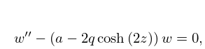
28.20.1 w ′′ − ( a − 2 ⁢ q ⁢ cosh ⁡ ( 2 ⁢ z ) ) ⁢ w = 0 ,
… ►
§28.20(ii) Solutions Ce ν , Se ν , Me ν , Fe n , Ge n
… ►
§28.20(iv) Radial Mathieu Functions Mc n ( j ) , Ms n ( j )
… ►
§28.20(vi) Wronskians
…
2: 28.21 Graphics
§28.21 Graphics
… ►
►
See accompanying text
►
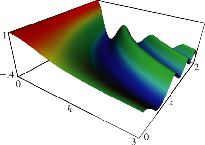
Figure 28.21.1: Mc 0 ( 1 ) ⁡ ( x , h ) for 0 ≤ h ≤ 3 , 0 ≤ x ≤ 2 . Magnify 3D Help
►
►
See accompanying text
►
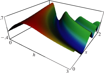
Figure 28.21.2: Mc 1 ( 1 ) ⁡ ( x , h ) for 0 ≤ h ≤ 3 , 0 ≤ x ≤ 2 . Magnify 3D Help
►
►
See accompanying text
►
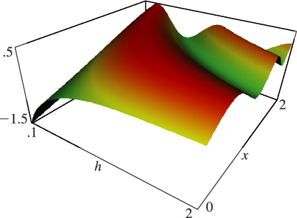
Figure 28.21.3: Mc 0 ( 2 ) ⁡ ( x , h ) for 0.1 ≤ h ≤ 2 , 0 ≤ x ≤ 2 . Magnify 3D Help
… ►
►
See accompanying text
►
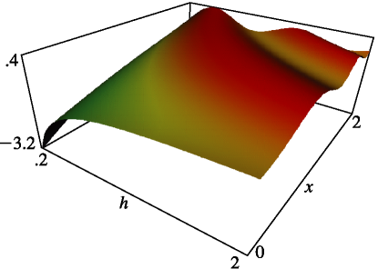
Figure 28.21.6: Ms 1 ( 2 ) ⁡ ( x , h ) for 0.2 ≤ h ≤ 2 , 0 ≤ x ≤ 2 . Magnify 3D Help
3: 10.26 Graphics
… ►
§10.26(i) Real Order and Variable
… ►
►See accompanying text►
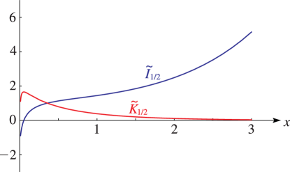
Figure 10.26.7: I ~ 1 / 2 ⁡ ( x ) , K ~ 1 / 2 ⁡ ( x ) , 0.01 ≤ x ≤ 3 . Magnify
►
►See accompanying text►
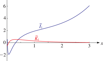
Figure 10.26.8: I ~ 1 ⁡ ( x ) , K ~ 1 ⁡ ( x ) , 0.01 ≤ x ≤ 3 . Magnify
►
►See accompanying text►
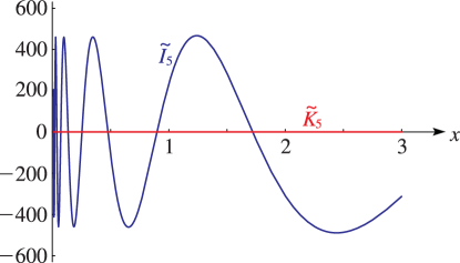
Figure 10.26.9: I ~ 5 ⁡ ( x ) , K ~ 5 ⁡ ( x ) , 0.01 ≤ x ≤ 3 . Magnify
►
►See accompanying text►
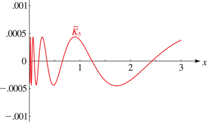
Figure 10.26.10: K ~ 5 ⁡ ( x ) , 0.01 ≤ x ≤ 3 . Magnify
4: 10.29 Recurrence Relations and Derivatives
… ►
§10.29(i) Recurrence Relations
►With 𝒵 ν ⁡ ( z ) defined as in §10.25(ii), … ►
I 0 ′ ⁡ ( z ) = I 1 ⁡ ( z ) ,
… ►For results on modified quotients of the form z ⁢ 𝒵 ν ± 1 ⁡ ( z ) / 𝒵 ν ⁡ ( z ) see Onoe (1955) and Onoe (1956). ►
§10.29(ii) Derivatives
…
5: 28.27 Addition Theorems
§28.27 Addition Theorems
… ►They are analogous to the addition theorems for Bessel functions (§10.23(ii)) and modified Bessel functions (§10.44(ii)). …
6: 10.28 Wronskians and Cross-Products
§10.28 Wronskians and Cross-Products
►
10.28.1 𝒲 ⁡ { I ν ⁡ ( z ) , I − ν ⁡ ( z ) } = I ν ⁡ ( z ) ⁢ I − ν − 1 ⁡ ( z ) − I ν + 1 ⁡ ( z ) ⁢ I − ν ⁡ ( z ) = − 2 ⁢ sin ⁡ ( ν ⁢ π ) / ( π ⁢ z ) ,
►
10.28.2 𝒲 ⁡ { K ν ⁡ ( z ) , I ν ⁡ ( z ) } = I ν ⁡ ( z ) ⁢ K ν + 1 ⁡ ( z ) + I ν + 1 ⁡ ( z ) ⁢ K ν ⁡ ( z ) = 1 / z .
7: 28.1 Special Notation
… ►and the modified Mathieu functions ► ►►►
Ce ν ⁡ ( z , q ) , Se ν ⁡ ( z , q ) , Fe n ⁡ ( z , q ) , Ge n ⁡ ( z , q ) ,
Me ν ⁡ ( z , q ) , M ν ( j ) ⁡ ( z , h ) , Mc n ( j ) ⁡ ( z , h ) , Ms n ( j ) ⁡ ( z , h ) ,
…
►The functions Mc n ( j ) ⁡ ( z , h ) and Ms n ( j ) ⁡ ( z , h ) are also known as the radial Mathieu functions. … ►The radial functions Mc n ( j ) ⁡ ( z , h ) and Ms n ( j ) ⁡ ( z , h ) are denoted by Mc n ( j ) ⁡ ( z , q ) and Ms n ( j ) ⁡ ( z , q ) , respectively.
8: 10.45 Functions of Imaginary Order
§10.45 Functions of Imaginary Order
… ►and I ~ ν ⁡ ( x ) , K ~ ν ⁡ ( x ) are real and linearly independent solutions of (10.45.1): … ►The corresponding result for K ~ ν ⁡ ( x ) is given by … ► … ►
9: 10.35 Generating Function and Associated Series
§10.35 Generating Function and Associated Series
… ►
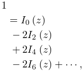
10.35.4 1 = I 0 ⁡ ( z ) − 2 ⁢ I 2 ⁡ ( z ) + 2 ⁢ I 4 ⁡ ( z ) − 2 ⁢ I 6 ⁡ ( z ) + ⋯ ,
►
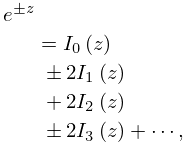
10.35.5 e ± z = I 0 ⁡ ( z ) ± 2 ⁢ I 1 ⁡ ( z ) + 2 ⁢ I 2 ⁡ ( z ) ± 2 ⁢ I 3 ⁡ ( z ) + ⋯ ,
►
cosh ⁡ z = I 0 ⁡ ( z ) + 2 ⁢ I 2 ⁡ ( z ) + 2 ⁢ I 4 ⁡ ( z ) + 2 ⁢ I 6 ⁡ ( z ) + … ,
►
sinh ⁡ z = 2 ⁢ I 1 ⁡ ( z ) + 2 ⁢ I 3 ⁡ ( z ) + 2 ⁢ I 5 ⁡ ( z ) + … .
10: 28.22 Connection Formulas
§28.22 Connection Formulas
… ►The joining factors in the above formulas are given by … ►
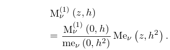
28.22.13 M ν ( 1 ) ⁡ ( z , h ) = M ν ( 1 ) ⁡ ( 0 , h ) me ν ⁡ ( 0 , h 2 ) ⁢ Me ν ⁡ ( z , h 2 ) .
►Here me ν ⁡ ( 0 , h 2 ) ( ≠ 0 ) is given by (28.14.1) with z = 0 , and M ν ( 1 ) ⁡ ( 0 , h ) is given by (28.24.1) with j = 1 , z = 0 , and n chosen so that | c 2 ⁢ n ν ⁡ ( h 2 ) | = max ⁡ ( | c 2 ⁢ ℓ ν ⁡ ( h 2 ) | ) , where the maximum is taken over all integers ℓ . … ►