mixed base Heine-type transformations

SearchAdvancedHelp

(0.003 seconds)

1—10 of 455 matching pages

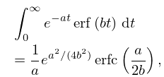
1: 1.14 Integral Transforms

§1.14 Integral Transforms

►

§1.14(i) Fourier Transform

… ►

§1.14(iii) Laplace Transform

… ►

Fourier Transform

… ►

Laplace Transform

…

2: 17.9 Further Transformations of ${}_{r+1}{}^{}\varphi _r^{}$ Functions

§17.9 Further Transformations of ${}_{r+1}{}^{}\varphi _r^{}$ Functions

… ►

F. H. Jackson’s Transformations

… ►

Transformations of ${}_3{}^{}\varphi _2^{}$-Series

… ►

Sears–Carlitz Transformation

… ►

Mixed-Base Heine-Type Transformations

…

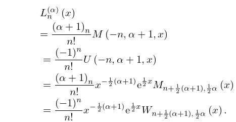
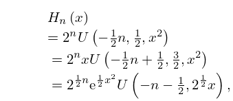
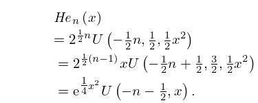
3: 18.11 Relations to Other Functions

… ►

18.11.2 $$L_n^{(\alpha )}\left(x\right)=\frac{{\left(\alpha +1\right)}_n}{n!}M(-n,\alpha +1,x)=\frac{{(-1)}^n}{n!}U(-n,\alpha +1,x)=\frac{{\left(\alpha +1\right)}_n}{n!}{x}^{-\frac{1}{2}(\alpha +1)}{\mathrm{e}}^{\frac{1}{2}x}{M}_{n+\frac{1}{2}(\alpha +1),\frac{1}{2}\alpha }\left(x\right)=\frac{{(-1)}^n}{n!}{x}^{-\frac{1}{2}(\alpha +1)}{\mathrm{e}}^{\frac{1}{2}x}{W}_{n+\frac{1}{2}(\alpha +1),\frac{1}{2}\alpha }\left(x\right).$$

ⓘ

Symbols:

$M(a,b,z)$: $={}_1{}^{}F_1^{}(a;b;z)$ Kummer confluent hypergeometric function, $U(a,b,z)$: Kummer confluent hypergeometric function, $L_n^{(\alpha )}\left(x\right)$: Laguerre (or generalized Laguerre) polynomial, ${\left(a\right)}_n$: Pochhammer’s symbol (or shifted factorial), $M_{\kappa ,\mu }\left(z\right)$: Whittaker confluent hypergeometric function, $W_{\kappa ,\mu }\left(z\right)$: Whittaker confluent hypergeometric function, $\mathrm{e}$: base of natural logarithm, $!$: factorial (as in $n!$), $n$: nonnegative integer and $x$: real variable

Referenced by:

§13.6(v), §18.11(i)

Permalink:

http://dlmf.nist.gov/18.11.E2

Encodings:

pMML, png, TeX

See also:

Annotations for §18.11(i), §18.11(i), §18.11 and Ch.18

… ►

18.11.3 $$H_n\left(x\right)=2^{n}U(-\frac{1}{2}n,\frac{1}{2},x^2)=2^{n}xU(-\frac{1}{2}n+\frac{1}{2},\frac{3}{2},x^2)=2^{\frac{1}{2}n}{\mathrm{e}}^{\frac{1}{2}{x}^2}U(-n-\frac{1}{2},2^{\frac{1}{2}}x),$$

ⓘ

Symbols:

$H_n\left(x\right)$: Hermite polynomial, $U(a,b,z)$: Kummer confluent hypergeometric function, $\mathrm{e}$: base of natural logarithm, $U(a,z)$: parabolic cylinder function, $n$: nonnegative integer and $x$: real variable

A&S Ref:

22.5.55, 22.5.58 ((factor $x$ missing on RHS of 22.5.55))

Referenced by:

§18.11(i), §18.15(v)

Permalink:

http://dlmf.nist.gov/18.11.E3

Encodings:

pMML, png, TeX

See also:

Annotations for §18.11(i), §18.11(i), §18.11 and Ch.18

►

18.11.4 $${\mathrm{𝐻𝑒}}_n\left(x\right)=2^{\frac{1}{2}n}U(-\frac{1}{2}n,\frac{1}{2},\frac{1}{2}{x}^2)=2^{\frac{1}{2}(n-1)}xU(-\frac{1}{2}n+\frac{1}{2},\frac{3}{2},\frac{1}{2}{x}^2)={\mathrm{e}}^{\frac{1}{4}{x}^2}U(-n-\frac{1}{2},x).$$

ⓘ

Symbols:

${\mathrm{𝐻𝑒}}_n\left(x\right)$: Hermite polynomial, $U(a,b,z)$: Kummer confluent hypergeometric function, $\mathrm{e}$: base of natural logarithm, $U(a,z)$: parabolic cylinder function, $n$: nonnegative integer and $x$: real variable

A&S Ref:

22.5.59

Permalink:

http://dlmf.nist.gov/18.11.E4

Encodings:

pMML, png, TeX

See also:

Annotations for §18.11(i), §18.11(i), §18.11 and Ch.18

… ►

§18.11(ii) Formulas of Mehler–Heine Type

…

4: 18.7 Interrelations and Limit Relations

… ►

§18.7(i) Linear Transformations

… ►

§18.7(ii) Quadratic Transformations

… ► See §18.11(ii) for limit formulas of Mehler–Heine type.

5: 1.18 Linear Second Order Differential Operators and Eigenfunction Expansions

… ►These are based on the Liouville normal form of (1.13.29). … ►

§1.18(viii) Mixed Spectra and Eigenfunction Expansions

… ► It is to be noted that if any of the $\lambda \in 𝝈$ have degenerate sub-spaces, that is subspaces of orthogonal eigenfunctions with identical eigenvalues, that in the expansions below all such distinct eigenfunctions are to be included. … ► See §18.39 for discussion of Schrödinger equations and operators. … …

6: 18.39 Applications in the Physical Sciences

… ►The properties of $V(x)$ determine whether the spectrum, this being the set of eigenvalues of $\mathscr{H}$, is discrete, continuous, or mixed, see §1.18. …Also presented are the analytic solutions for the $L^2$, bound state, eigenfunctions and eigenvalues of the Morse oscillator which also has analytically known non-normalizable continuum eigenfunctions, thus providing an example of a mixed spectrum. … ►Brief mention of non-unit normalized solutions in the case of mixed spectra appear, but as these solutions are not OP’s details appear elsewhere, as referenced. … ►The spectrum is mixed, as in §1.18(viii), the positive energy, non-$L^2$, scattering states are the subject of Chapter 33. … ►Namely for fixed $l$ the infinite set labeled by $p$ describe only the $L^2$ bound states for that single $l$, omitting the continuum briefly mentioned below, and which is the subject of Chapter 33, and so an unusual example of the mixed spectra of §1.18(viii). …

7: 1.13 Differential Equations

… ►

Transformation of the Point at Infinity

… ►

Liouville Transformation

… ►Assuming that $u(x)$ satisfies un-mixed boundary conditions of the form … ►

Transformation to Liouville normal Form

… ►For a regular Sturm-Liouville system, equations (1.13.26) and (1.13.29) have: (i) identical eigenvalues, $\lambda$; (ii) the corresponding (real) eigenfunctions, $u(x)$ and $w(t)$, have the same number of zeros, also called nodes, for $t\in (0,c)$ as for $x\in (a,b)$; (iii) the eigenfunctions also satisfy the same type of boundary conditions, un-mixed or periodic, for both forms at the corresponding boundary points. …

8: Bibliography S

… ►

Adaptive Quasi-Monte Carlo Integration Based on MISER and VEGAS. In Monte Carlo and Quasi-Monte Carlo Methods 2002, pp. 393–406.

ⓘ

External Links:

MathReview Entry, ZentralBlatt

Referenced by:

§3.5(x).

Encodings:

BibTeX

… ►

A code to evaluate modified Bessel functions based on the continued fraction method. Comput. Phys. Comm. 105 (2-3), pp. 263–272.

ⓘ

External Links:

ISSN 0010-4655, Document, Code, MathReview, ZentralBlatt

Referenced by:

7th item.

Encodings:

BibTeX

… ►

Special Functions: A Unified Theory Based on Singularities. Oxford Mathematical Monographs, Oxford University Press, Oxford.

ⓘ

External Links:

ISBN 0-19-850573-6, MathReview, ZentralBlatt

Referenced by:

Ch.2, §31.12, §31.17(ii).

Encodings:

BibTeX

… ►

Mixed Boundary Value Problems in Potential Theory. North-Holland Publishing Co., Amsterdam.

ⓘ

External Links:

MathReview (R. Shail), ZentralBlatt

Referenced by:

§10.22(iv).

Encodings:

BibTeX

… ►

Numerical Methods Based on Sinc and Analytic Functions. Springer Series in Computational Mathematics, Vol. 20, Springer-Verlag, New York.

ⓘ

Notes:

Sinc-Pack, a set of 480 Matlab programs with a 470-page tutorial, is available for purchase from SINC, LLC by contacting Frank Stenger.

External Links:

ISBN 0-387-94008-1, MathReview (B. Boyanov), ZentralBlatt

Referenced by:

§3.3(vi), §3.4(i), §3.5(i).

Encodings:

BibTeX

…

9: 2.5 Mellin Transform Methods

§2.5 Mellin Transform Methods

… ►The Mellin transform of $f(t)$ is defined by …The inversion formula is given by … ► … ►

§2.5(iii) Laplace Transforms with Small Parameters

…

10: 7.14 Integrals

… ►

Fourier Transform

… ►

Laplace Transforms

►

7.14.2 $${\int }_0^{\mathrm{\infty }}{\mathrm{e}}^{-at}\mathrm{erf}\left(bt\right)dt=\frac{1}{a}{\mathrm{e}}^{a^2/(4b^2)}\mathrm{erfc}\left(\frac{a}{2b}\right),$$ $\mathrm{\Re }a>0$, ,

ⓘ

Symbols:

$\pi$: the ratio of the circumference of a circle to its diameter, $\mathrm{erfc}z$: complementary error function, $dx$: differential of $x$ , $\mathrm{erf}z$: error function, $\mathrm{e}$: base of natural logarithm, $\int$: integral, $\mathrm{ph}$: phase and $\mathrm{\Re }$: real part

Keywords:

Laplace transform

A&S Ref:

7.4.17

Referenced by:

§7.14(i)

Permalink:

http://dlmf.nist.gov/7.14.E2

Encodings:

pMML, png, TeX

See also:

Annotations for §7.14(i), §7.14(i), §7.14 and Ch.7

►

7.14.3 $${\int }_0^{\mathrm{\infty }}{\mathrm{e}}^{-at}\mathrm{erf}\sqrt{bt}dt=\frac{1}{a}\sqrt{\frac{b}{a+b}},$$ $\mathrm{\Re }a>0$, $\mathrm{\Re }b>0$,

ⓘ

Symbols:

$dx$: differential of $x$ , $\mathrm{erf}z$: error function, $\mathrm{e}$: base of natural logarithm, $\int$: integral and $\mathrm{\Re }$: real part

Keywords:

Laplace transform

A&S Ref:

7.4.19

Referenced by:

§7.14(i)

Permalink:

http://dlmf.nist.gov/7.14.E3

Encodings:

pMML, png, TeX

See also:

Annotations for §7.14(i), §7.14(i), §7.14 and Ch.7

… ►

Laplace Transforms

…