logarithmic%20integral

SearchAdvancedHelp

(0.004 seconds)

1—10 of 26 matching pages

1: 6.16 Mathematical Applications

… ►

►►

Figure 6.16.2: The logarithmic integral $\mathrm{li}\left(x\right)$, together with vertical bars indicating the value of $\pi (x)$ for $x=10,20,\mathrm{\dots },1000$. Magnify

2: 6.19 Tables

… ►

Abramowitz and Stegun (1964, Chapter 5) includes the real and imaginary parts of $z{\mathrm{e}}^z{E}_1\left(z\right)$, $x=-19(1)20$, $y=0(1)20$, 6D; ${\mathrm{e}}^z{E}_1\left(z\right)$, $x=-4(.5)-2$, $y=0(.2)1$, 6D; $E_1\left(z\right)+\ln z$, $x=-2(.5)2.5$, $y=0(.2)1$, 6D.

…

3: 6.20 Approximations

… ►

Hastings (1955) gives several minimax polynomial and rational approximations for $E_1\left(x\right)+\ln x$, $x{\mathrm{e}}^x{E}_1\left(x\right)$, and the auxiliary functions $\mathrm{f}\left(x\right)$ and $\mathrm{g}\left(x\right)$. These are included in Abramowitz and Stegun (1964, Ch. 5).

►

Cody and Thacher (1968) provides minimax rational approximations for $E_1\left(x\right)$, with accuracies up to 20S.

►

Cody and Thacher (1969) provides minimax rational approximations for $\mathrm{Ei}\left(x\right)$, with accuracies up to 20S.

►

MacLeod (1996b) provides rational approximations for the sine and cosine integrals and for the auxiliary functions $\mathrm{f}$ and $\mathrm{g}$, with accuracies up to 20S.

… ►

Clenshaw (1962) gives Chebyshev coefficients for $-E_1\left(x\right)-\ln |x|$ for $-4\le x\le 4$ and ${\mathrm{e}}^x{E}_1\left(x\right)$ for $x\ge 4$ (20D).

…

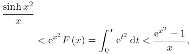
4: 7.8 Inequalities

… ►

7.8.1 $$𝖬\left(x\right)=\frac{{\int }_x^{\mathrm{\infty }}{\mathrm{e}}^{-t^2}dt}{{\mathrm{e}}^{-x^2}}={\mathrm{e}}^{x^2}{\int }_x^{\mathrm{\infty }}{\mathrm{e}}^{-t^2}dt.$$

ⓘ

Defines:

$𝖬\left(x\right)$: Mills’ ratio

Symbols:

$dx$: differential of $x$ , $\mathrm{e}$: base of natural logarithm, $\int$: integral and $x$: real variable

Permalink:

http://dlmf.nist.gov/7.8.E1

Encodings:

pMML, png, TeX

See also:

Annotations for §7.8 and Ch.7

… ►

7.8.6 $a,x>0$.

ⓘ

Symbols:

$dx$: differential of $x$ , $\mathrm{e}$: base of natural logarithm, $\int$: integral and $x$: real variable

Referenced by:

§7.8

Permalink:

http://dlmf.nist.gov/7.8.E6

Encodings:

pMML, png, TeX

See also:

Annotations for §7.8 and Ch.7

►

7.8.7 $x>0$.

ⓘ

Symbols:

$F\left(z\right)$: Dawson’s integral, $dx$: differential of $x$ , $\mathrm{e}$: base of natural logarithm, $\sinh z$: hyperbolic sine function, $\int$: integral and $x$: real variable

Referenced by:

Erratum (V1.1.5) for Additions

Permalink:

http://dlmf.nist.gov/7.8.E7

Encodings:

pMML, png, TeX

Addition (effective with 1.1.5):

A new inequality was added.

See also:

Annotations for §7.8 and Ch.7

►The function $F\left(x\right)/\sqrt{1-{\mathrm{e}}^{-2x^2}}$ is strictly decreasing for $x>0$. For these and similar results for Dawson’s integral $F\left(x\right)$ see Janssen (2021). …

5: Bibliography M

… ►

Rational approximations, software and test methods for sine and cosine integrals. Numer. Algorithms 12 (3-4), pp. 259–272.

ⓘ

Notes:

Includes Fortran code, maximum accuracy 20S.

External Links:

ISSN 1017-1398, Document, MathReview, ZentralBlatt

Referenced by:

§6.13, 4th item, §6.21(ii).

Encodings:

BibTeX

… ►

Hill’s Equation. Interscience Tracts in Pure and Applied Mathematics, No. 20, Interscience Publishers John Wiley & Sons, New York-London-Sydney.

ⓘ

Notes:

Reprinted by Dover Publications, Inc., New York, 1979.

External Links:

MathReview (H. Hochstadt), ZentralBlatt

Referenced by:

§1.3(iii), §28.29(i), §28.29(ii), §28.29(ii), §28.29(iii), §28.29(iii), §28.29(iii), §28.30(i), Ch.28, §29.3(i), §29.9.

Encodings:

BibTeX

… ►

Calculation of the modified Bessel functions of the second kind with complex argument. Math. Comp. 20 (95), pp. 407–412.

ⓘ

External Links:

ISSN 0025-5718, FullText, MathReview (H. E. Fettis), ZentralBlatt

Referenced by:

§10.74(iii).

Encodings:

BibTeX

… ►

Hierarchies and logarithmic oscillations in the temporal relaxation patterns of proteins and other complex systems. Proc. Nat. Acad. Sci. U .S. A. 96 (20), pp. 11085–11089.

ⓘ

External Links:

FullText

Referenced by:

§8.24(i).

Encodings:

BibTeX

… ►

The $q$-analogue of the Laguerre polynomials. J. Math. Anal. Appl. 81 (1), pp. 20–47.

ⓘ

External Links:

ISSN 0022-247X, Document, MathReview (R. A. Askey), ZentralBlatt

Referenced by:

§18.27(v).

Encodings:

BibTeX

…

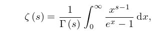
6: 25.12 Polylogarithms

… ►The right-hand side is called Clausen’s integral. … ►

Integral Representation

… ►

§25.12(iii) Fermi–Dirac and Bose–Einstein Integrals

►The Fermi–Dirac and Bose–Einstein integrals are defined by … ►In terms of polylogarithms …

7: 25.20 Approximations

… ►

Cody et al. (1971) gives rational approximations for $\zeta \left(s\right)$ in the form of quotients of polynomials or quotients of Chebyshev series. The ranges covered are $0.5\le s\le 5$, $5\le s\le 11$, $11\le s\le 25$, $25\le s\le 55$. Precision is varied, with a maximum of 20S.

… ►

Luke (1969b, p. 306) gives coefficients in Chebyshev-series expansions that cover $\zeta \left(s\right)$ for $0\le s\le 1$ (15D), $\zeta \left(s+1\right)$ for $0\le s\le 1$ (20D), and $\ln \xi \left(\frac{1}{2}+\mathrm{i}x\right)$ (§25.4) for $-1\le x\le 1$ (20D). For errata see Piessens and Branders (1972).

►

Morris (1979) gives rational approximations for ${\mathrm{Li}}_2\left(x\right)$ (§25.12(i)) for $0.5\le x\le 1$. Precision is varied with a maximum of 24S.

►

Antia (1993) gives minimax rational approximations for $\mathrm{\Gamma }\left(s+1\right)F_s(x)$, where $F_s(x)$ is the Fermi–Dirac integral (25.12.14), for the intervals and , with $s=-\frac{1}{2},\frac{1}{2},\frac{3}{2},\frac{5}{2}$. For each $s$ there are three sets of approximations, with relative maximum errors ${10}^{-4},{10}^{-8},{10}^{-12}$.

8: 25.5 Integral Representations

§25.5 Integral Representations

… ►

25.5.1 $$\zeta \left(s\right)=\frac{1}{\mathrm{\Gamma }\left(s\right)}{\int }_0^{\mathrm{\infty }}\frac{x^{s-1}}{{\mathrm{e}}^x-1}dx,$$ $\mathrm{\Re }s>1$.

ⓘ

Symbols:

$\mathrm{\Gamma }\left(z\right)$: gamma function, $\zeta \left(s\right)$: Riemann zeta function, $dx$: differential of $x$ , $\mathrm{e}$: base of natural logarithm, $\int$: integral, $\mathrm{\Re }$: real part, $x$: real variable and $s$: complex variable

Keywords:

improper integral, integral representation

Source:

Erdélyi et al. (1953a, (1.12.4), p. 32)

A&S Ref:

23.2.7

Referenced by:

§25.12(ii), (25.5.2), (25.5.6)

Permalink:

http://dlmf.nist.gov/25.5.E1

Encodings:

pMML, png, TeX

See also:

Annotations for §25.5(i), §25.5 and Ch.25

►

25.5.2 $$\zeta \left(s\right)=\frac{1}{\mathrm{\Gamma }\left(s+1\right)}{\int }_0^{\mathrm{\infty }}\frac{{\mathrm{e}}^x{x}^s}{{({\mathrm{e}}^x-1)}^2}dx,$$ $\mathrm{\Re }s>1$.

ⓘ

Symbols:

$\mathrm{\Gamma }\left(z\right)$: gamma function, $\zeta \left(s\right)$: Riemann zeta function, $dx$: differential of $x$ , $\mathrm{e}$: base of natural logarithm, $\int$: integral, $\mathrm{\Re }$: real part, $x$: real variable and $s$: complex variable

Keywords:

improper integral, integral representation

Proof sketch:

Derivable from (25.5.1) by integration by parts.

Permalink:

http://dlmf.nist.gov/25.5.E2

Encodings:

pMML, png, TeX

See also:

Annotations for §25.5(i), §25.5 and Ch.25

… ►

25.5.15 $$\zeta \left(s\right)=\frac{1}{s-1}+\frac{\sin \left(\pi s\right)}{\pi }{\int }_0^{\mathrm{\infty }}(\ln \left(1+x\right)-\psi \left(1+x\right))x^{-s}dx,$$

ⓘ

Symbols:

$\zeta \left(s\right)$: Riemann zeta function, $\pi$: the ratio of the circumference of a circle to its diameter, $dx$: differential of $x$ , $\psi \left(z\right)$: psi (or digamma) function, $\int$: integral, $\ln z$: principal branch of logarithm function, $\sin z$: sine function, $x$: real variable and $s$: complex variable

Keywords:

improper integral, integral representation

Source:

de Bruijn (1937, (18), p. 175)

Referenced by:

§25.5(ii)

Permalink:

http://dlmf.nist.gov/25.5.E15

Encodings:

pMML, png, TeX

See also:

Annotations for §25.5(ii), §25.5 and Ch.25

… ►

§25.5(iii) Contour Integrals

…

9: 20.10 Integrals

§20.10 Integrals

… ►

20.10.1 $${\int }_0^{\mathrm{\infty }}{x}^{s-1}{\theta }_2\left(0\right|\mathrm{i}{x}^2)dx=2^s(1-2^{-s}){\pi }^{-s/2}\mathrm{\Gamma }\left(\frac{1}{2}s\right)\zeta \left(s\right),$$ $\mathrm{\Re }s>1$,

ⓘ

Symbols:

$\mathrm{\Gamma }\left(z\right)$: gamma function, ${\theta }_j\left(z\right|\tau )$: theta function, $\zeta \left(s\right)$: Riemann zeta function, $\pi$: the ratio of the circumference of a circle to its diameter, $dx$: differential of $x$ , $\mathrm{i}$: imaginary unit, $\int$: integral and $\mathrm{\Re }$: real part

Keywords:

Mellin transform

Referenced by:

§20.10(i), Erratum (V1.1.5) for §20.10(i)

Permalink:

http://dlmf.nist.gov/20.10.E1

Encodings:

pMML, png, TeX

Modification (effective with 1.1.5):

Originally the constraint was $\mathrm{\Re }s>2$. This can be relaxed to $\mathrm{\Re }s>1$ because ${\theta }_2\left(0\right|\mathrm{i}{x}^2)=x^{-1}{\theta }_4\left(0\right|\mathrm{i}{x}^{-2})\sim x^{-1}$ as $x\to 0+$, which follows from (20.7.31) and (20.4.5).

See also:

Annotations for §20.10(i), §20.10 and Ch.20

… ►

20.10.4 $${\int }_0^{\mathrm{\infty }}{\mathrm{e}}^{-st}{\theta }_1\left(\frac{\beta \pi }{2\mathrm{\ell }}\right|\frac{\mathrm{i}\pi t}{{\mathrm{\ell }}^2})dt={\int }_0^{\mathrm{\infty }}{\mathrm{e}}^{-st}{\theta }_2\left(\frac{(1+\beta )\pi }{2\mathrm{\ell }}\right|\frac{\mathrm{i}\pi t}{{\mathrm{\ell }}^2})dt=-\frac{\mathrm{\ell }}{\sqrt{s}}\sinh \left(\beta \sqrt{s}\right)\mathrm{sech}\left(\mathrm{\ell }\sqrt{s}\right),$$

ⓘ

Symbols:

${\theta }_j\left(z\right|\tau )$: theta function, $\pi$: the ratio of the circumference of a circle to its diameter, $dx$: differential of $x$ , $\mathrm{e}$: base of natural logarithm, $\mathrm{sech}z$: hyperbolic secant function, $\sinh z$: hyperbolic sine function, $\mathrm{i}$: imaginary unit, $\int$: integral, $s$: parameter, $\beta$: parameter and $\mathrm{\ell }$: parameter

Permalink:

http://dlmf.nist.gov/20.10.E4

Encodings:

pMML, png, TeX

See also:

Annotations for §20.10(ii), §20.10 and Ch.20

►

20.10.5 $${\int }_0^{\mathrm{\infty }}{\mathrm{e}}^{-st}{\theta }_3\left(\frac{(1+\beta )\pi }{2\mathrm{\ell }}\right|\frac{\mathrm{i}\pi t}{{\mathrm{\ell }}^2})dt={\int }_0^{\mathrm{\infty }}{\mathrm{e}}^{-st}{\theta }_4\left(\frac{\beta \pi }{2\mathrm{\ell }}\right|\frac{\mathrm{i}\pi t}{{\mathrm{\ell }}^2})dt=\frac{\mathrm{\ell }}{\sqrt{s}}\cosh \left(\beta \sqrt{s}\right)\mathrm{csch}\left(\mathrm{\ell }\sqrt{s}\right).$$

ⓘ

Symbols:

${\theta }_j\left(z\right|\tau )$: theta function, $\pi$: the ratio of the circumference of a circle to its diameter, $dx$: differential of $x$ , $\mathrm{e}$: base of natural logarithm, $\mathrm{csch}z$: hyperbolic cosecant function, $\cosh z$: hyperbolic cosine function, $\mathrm{i}$: imaginary unit, $\int$: integral, $s$: parameter, $\beta$: parameter and $\mathrm{\ell }$: parameter

Permalink:

http://dlmf.nist.gov/20.10.E5

Encodings:

pMML, png, TeX

See also:

Annotations for §20.10(ii), §20.10 and Ch.20

… ►For further integrals of theta functions see Erdélyi et al. (1954a, pp. 61–62 and 339), Prudnikov et al. (1990, pp. 356–358), Prudnikov et al. (1992a, §3.41), and Gradshteyn and Ryzhik (2000, pp. 627–628).

10: 11.14 Tables

… ►

Zhang and Jin (1996) tabulates ${𝐇}_n\left(x\right)$ and ${𝐋}_n\left(x\right)$ for $n=-4(1)3$ and $x=0(1)20$ to 8D or 7S.

►

§11.14(iii) Integrals

►

Abramowitz and Stegun (1964, Chapter 12) tabulates ${\int }_0^x(I_0\left(t\right)-{𝐋}_0\left(t\right))dt$ and $(2/\pi ){\int }_x^{\mathrm{\infty }}{t}^{-1}{𝐇}_0\left(t\right)dt$ for $x=0(.1)5$ to 5D or 7D; ${\int }_0^x({𝐇}_0\left(t\right)-Y_0\left(t\right))dt-(2/\pi )\ln x$, ${\int }_0^x(I_0\left(t\right)-{𝐋}_0\left(t\right))dt-(2/\pi )\ln x$, and ${\int }_x^{\mathrm{\infty }}{t}^{-1}({𝐇}_0\left(t\right)-Y_0\left(t\right))dt$ for $x^{-1}=0(.01)0.2$ to 6D.

►

Agrest et al. (1982) tabulates ${\int }_0^x{𝐇}_0\left(t\right)dt$ and ${\mathrm{e}}^{-x}{\int }_0^x{𝐋}_0\left(t\right)dt$ for $x=0(.001)5(.005)15(.01)100$ to 11D.

…