locally integrable

SearchAdvancedHelp

(0.002 seconds)

21—30 of 39 matching pages

21: 2.4 Contour Integrals

… ►If $q(t)$ is analytic in a sector containing $\mathrm{ph}t=0$, then the region of validity may be increased by rotation of the integration paths. … ►On the interval let $q(t)$ be differentiable and ${\mathrm{e}}^{-ct}q(t)$ be absolutely integrable, where $c$ is a real constant. … ►Then by integration by parts the integral … ►The most successful results are obtained on moving the integration contour as far to the left as possible. … ►The change of integration variable is given by …

22: 3.7 Ordinary Differential Equations

… ►

3.7.1 $$\frac{d^{2}w}{{dz}^2}+f(z)\frac{dw}{dz}+g(z)w=h(z),$$

ⓘ

Defines:

$f(z)$: function (locally), $g(z)$: function (locally) and $h(z)$: function (locally)

Symbols:

$\frac{df}{dx}$: derivative of $f$ with respect to $x$ and $w(z)$: function

Referenced by:

§3.7(i), §3.7(ii), §3.7(ii), §3.7(ii)

Permalink:

http://dlmf.nist.gov/3.7.E1

Encodings:

pMML, png, TeX

See also:

Annotations for §3.7(i), §3.7 and Ch.3

… ►Assume that we wish to integrate (3.7.1) along a finite path $𝒫$ from $z=a$ to $z=b$ in a domain $D$. … ►

3.7.6

ⓘ

Defines:

$𝐀(\tau ,z)$: matrix (locally) and $A_{jk}(\tau ,z)$: matrix entry (locally)

Permalink:

http://dlmf.nist.gov/3.7.E6

Encodings:

pMML, png, TeX

See also:

Annotations for §3.7(ii), §3.7 and Ch.3

… ►

3.7.7 $$𝐛(\tau ,z)=\left[\begin{array}{c}{b}_1(\tau ,z)\\ b_2(\tau ,z)\end{array}\right],$$

ⓘ

Defines:

$𝐛(\tau ,z)$: vector (locally) and $b_j(\tau ,z)$: vector (locally)

Permalink:

http://dlmf.nist.gov/3.7.E7

Encodings:

pMML, png, TeX

See also:

Annotations for §3.7(ii), §3.7 and Ch.3

… ►The larger the absolute values of the eigenvalues ${\lambda }_k$ that are being sought, the smaller the integration steps $\left|{\tau }_j\right|$ need to be. …

23: 18.38 Mathematical Applications

… ►If the nodes in a quadrature formula with a positive weight function are chosen to be the zeros of the $n$th degree OP with the same weight function, and the interval of orthogonality is the same as the integration range, then the weights in the quadrature formula can be chosen in such a way that the formula is exact for all polynomials of degree not exceeding $2n-1$. … ►The terminology DVR arises as an otherwise continuous variable, such as the co-ordinate $x$, is replaced by its values at a finite set of zeros of appropriate OP’s resulting in expansions using functions localized at these points. … ►

Integrable Systems

►The Toda equation provides an important model of a completely integrable system. …

24: 18.18 Sums

… ►

18.18.1 $$a_n=\frac{n!(2n+\alpha +\beta +1)\mathrm{\Gamma }\left(n+\alpha +\beta +1\right)}{2^{\alpha +\beta +1}\mathrm{\Gamma }\left(n+\alpha +1\right)\mathrm{\Gamma }\left(n+\beta +1\right)}{\int }_{-1}^{1}f(x)P_n^{(\alpha ,\beta )}\left(x\right){(1-x)}^{\alpha }{(1+x)}^{\beta }dx.$$

ⓘ

Defines:

$a_n$ (locally)

Symbols:

$\mathrm{\Gamma }\left(z\right)$: gamma function, $P_n^{(\alpha ,\beta )}\left(x\right)$: Jacobi polynomial, $dx$: differential of $x$ , $!$: factorial (as in $n!$), $\int$: integral, $n$: nonnegative integer, $f(z)$: analytic function and $x$: real variable

Referenced by:

§18.18(i), §18.18(i)

Permalink:

http://dlmf.nist.gov/18.18.E1

Encodings:

pMML, png, TeX

See also:

Annotations for §18.18(i), §18.18(i), §18.18 and Ch.18

… ►

18.18.7 $$d_n=\frac{1}{\sqrt{\pi }{2}^{n}n!}{\int }_{-\mathrm{\infty }}^{\mathrm{\infty }}f(x)H_n\left(x\right){\mathrm{e}}^{-x^2}dx.$$

ⓘ

Defines:

$d_n$ (locally)

Symbols:

$H_n\left(x\right)$: Hermite polynomial, $\pi$: the ratio of the circumference of a circle to its diameter, $dx$: differential of $x$ , $\mathrm{e}$: base of natural logarithm, $!$: factorial (as in $n!$), $\int$: integral, $n$: nonnegative integer, $f(z)$: analytic function and $x$: real variable

Referenced by:

§18.18(i)

Permalink:

http://dlmf.nist.gov/18.18.E7

Encodings:

pMML, png, TeX

See also:

Annotations for §18.18(i), §18.18(i), §18.18 and Ch.18

… ►

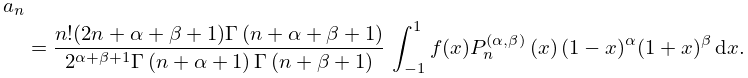
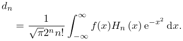
Expansion of $L^2$ functions

►In all three cases of Jacobi, Laguerre and Hermite, if $f(x)$ is $L^2$ on the corresponding interval with respect to the corresponding weight function and if $a_n,b_n,d_n$ are given by (18.18.1), (18.18.5), (18.18.7), respectively, then the respective series expansions (18.18.2), (18.18.4), (18.18.6) are valid with the sums converging in $L^2$ sense. … ►See (18.17.45) and (18.17.49) for integrated forms of (18.18.22) and (18.18.23), respectively. …

25: 13.29 Methods of Computation

… ►A comprehensive and powerful approach is to integrate the differential equations (13.2.1) and (13.14.1) by direct numerical methods. As described in §3.7(ii), to insure stability the integration path must be chosen in such a way that as we proceed along it the wanted solution grows in magnitude at least as fast as all other solutions of the differential equation. ►For $M(a,b,z)$ and $M_{\kappa ,\mu }\left(z\right)$ this means that in the sector $|\mathrm{ph}z|\le \pi$ we may integrate along outward rays from the origin with initial values obtained from (13.2.2) and (13.14.2). … ►In the sector the integration has to be towards the origin, with starting values computed from asymptotic expansions (§§13.7 and 13.19). On the rays $\mathrm{ph}z=\pm \frac{1}{2}\pi$, integration can proceed in either direction. …

26: 1.15 Summability Methods

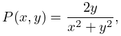
… ►If $f(\theta )$ is periodic and integrable on $[0,2\pi ]$, then as $n\to \mathrm{\infty }$ the Abel means $A(r,\theta )$ and the (C,1) means ${\sigma }_n(\theta )$ converge to … ►

1.15.33 $$P(x,y)=\frac{2y}{x^2+y^2},$$ $y>0$, .

ⓘ

Defines:

$P(x,y)$: Poisson kernel (locally)

Permalink:

http://dlmf.nist.gov/1.15.E33

Encodings:

pMML, png, TeX

See also:

Annotations for §1.15(v), §1.15(v), §1.15 and Ch.1

… ►If $f(x)$ is integrable on $(-\mathrm{\infty },\mathrm{\infty })$, then … ►Suppose now $f(x)$ is real-valued and integrable on $(-\mathrm{\infty },\mathrm{\infty })$. … ►If $f(\theta )$ is integrable on $(-\mathrm{\infty },\mathrm{\infty })$, then …

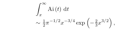
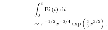
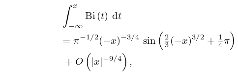
27: 9.10 Integrals

… ►

9.10.4 $${\int }_x^{\mathrm{\infty }}\mathrm{Ai}\left(t\right)dt\sim \frac{1}{2}{\pi }^{-1/2}{x}^{-3/4}\exp \left(-\frac{2}{3}{x}^{3/2}\right),$$ $x\to \mathrm{\infty }$,

ⓘ

Symbols:

$\mathrm{Ai}\left(z\right)$: Airy function, $\sim$: asymptotic equality, $\pi$: the ratio of the circumference of a circle to its diameter, $dx$: differential of $x$ , $\exp z$: exponential function, $\int$: integral and $x$: real variable

Proof sketch:

Integrate the leading term of (9.7.5).

Referenced by:

§9.10(ii)

Permalink:

http://dlmf.nist.gov/9.10.E4

Encodings:

pMML, png, TeX

See also:

Annotations for §9.10(ii), §9.10 and Ch.9

►

9.10.5 $${\int }_0^x\mathrm{Bi}\left(t\right)dt\sim {\pi }^{-1/2}{x}^{-3/4}\exp \left(\frac{2}{3}{x}^{3/2}\right),$$ $x\to \mathrm{\infty }$.

ⓘ

Symbols:

$\mathrm{Bi}\left(z\right)$: Airy function, $\sim$: asymptotic equality, $\pi$: the ratio of the circumference of a circle to its diameter, $dx$: differential of $x$ , $\exp z$: exponential function, $\int$: integral and $x$: real variable

Proof sketch:

Integrate the leading term of (9.7.7).

Permalink:

http://dlmf.nist.gov/9.10.E5

Encodings:

pMML, png, TeX

See also:

Annotations for §9.10(ii), §9.10 and Ch.9

►

9.10.6 $${\int }_{-\mathrm{\infty }}^x\mathrm{Ai}\left(t\right)dt={\pi }^{-1/2}{(-x)}^{-3/4}\cos \left(\frac{2}{3}{(-x)}^{3/2}+\frac{1}{4}\pi \right)+O\left({|x|}^{-9/4}\right),$$ $x\to -\mathrm{\infty }$,

ⓘ

Symbols:

$\mathrm{Ai}\left(z\right)$: Airy function, $O\left(x\right)$: order not exceeding, $\pi$: the ratio of the circumference of a circle to its diameter, $\cos z$: cosine function, $dx$: differential of $x$ , $\int$: integral and $x$: real variable

Proof sketch:

Integrate the leading terms of (9.7.5) and use (9.10.11)

Permalink:

http://dlmf.nist.gov/9.10.E6

Encodings:

pMML, png, TeX

See also:

Annotations for §9.10(ii), §9.10 and Ch.9

►

9.10.7 $${\int }_{-\mathrm{\infty }}^x\mathrm{Bi}\left(t\right)dt={\pi }^{-1/2}{(-x)}^{-3/4}\sin \left(\frac{2}{3}{(-x)}^{3/2}+\frac{1}{4}\pi \right)+O\left({|x|}^{-9/4}\right),$$ $x\to -\mathrm{\infty }$.

ⓘ

Symbols:

$\mathrm{Bi}\left(z\right)$: Airy function, $O\left(x\right)$: order not exceeding, $\pi$: the ratio of the circumference of a circle to its diameter, $dx$: differential of $x$ , $\int$: integral, $\sin z$: sine function and $x$: real variable

Proof sketch:

Integrate the leading terms of (9.7.7) and use (9.10.12)

Referenced by:

§9.10(ii)

Permalink:

http://dlmf.nist.gov/9.10.E7

Encodings:

pMML, png, TeX

See also:

Annotations for §9.10(ii), §9.10 and Ch.9

… ►

9.10.10 $$\int z^{n+3}w(z)dz=z^{n+2}{w}^{\prime }(z)-(n+2)z^{n+1}w(z)+(n+1)(n+2)\int z^{n}w(z)dz,$$ $n=0,1,2,\mathrm{\dots }.$

ⓘ

Defines:

$n$: index (locally)

Symbols:

$dx$: differential of $x$ , $\int$: integral, $z$: complex variable and $w$: ODE solution

Proof sketch:

To verify, differentiate and refer to (9.2.1).

Permalink:

http://dlmf.nist.gov/9.10.E10

Encodings:

pMML, png, TeX

See also:

Annotations for §9.10(iii), §9.10 and Ch.9

…

28: 10.43 Integrals

… ►

10.43.30 $$f(y)=\frac{2y}{{\pi }^2}\sinh \left(\pi y\right){\int }_0^{\mathrm{\infty }}\frac{g(x)}{x}{K}_{\mathrm{i}y}\left(x\right)dx.$$

ⓘ

Defines:

$f(x)$: Kontorovich–Lebedev transform of $g(x)$ (locally)

Symbols:

$\pi$: the ratio of the circumference of a circle to its diameter, $dx$: differential of $x$ , $\sinh z$: hyperbolic sine function, $\mathrm{i}$: imaginary unit, $\int$: integral, $K_{\nu }\left(z\right)$: modified Bessel function of the second kind, $x$: real variable, $y$: real variable and $g(x)$: function

Referenced by:

§10.43(v)

Permalink:

http://dlmf.nist.gov/10.43.E30

Encodings:

pMML, png, TeX

See also:

Annotations for §10.43(v), §10.43 and Ch.10

… ►

On the interval , $x^{-1}g(x)$ is continuously differentiable and each of $xg(x)$ and $xd(x^{-1}g(x))/dx$ is absolutely integrable.

…

29: 1.6 Vectors and Vector-Valued Functions

… ►If $h(a)=a^{\prime }$ and $h(b)=b^{\prime }$, then the reparametrization is called orientation-preserving, and …If $h(a)=b^{\prime }$ and $h(b)=a^{\prime }$, then the reparametrization is orientation-reversing and … ►

1.6.43 $$𝐅(x,y)=F_1(x,y)𝐢+F_2(x,y)𝐣$$

ⓘ

Defines:

$𝐅(x,y)$: vector (locally)

Symbols:

$𝐢$: unit vector, $𝐣$: unit vector and $F_j$: vector function components

Permalink:

http://dlmf.nist.gov/1.6.E43

Encodings:

pMML, png, TeX

See also:

Annotations for §1.6(iv), §1.6(iv), §1.6 and Ch.1

… ►

1.6.45 $$𝚽(u,v)=(x(u,v),y(u,v),z(u,v))$$

ⓘ

Defines:

$𝚽(x,y,z)$: parameterization (locally)

Symbols:

$(a,b)$: open interval

Permalink:

http://dlmf.nist.gov/1.6.E45

Encodings:

pMML, png, TeX

See also:

Annotations for §1.6(v), §1.6 and Ch.1

… ►

1.6.48 $$A(S)={\iint }_D\Vert {𝐓}_u\times {𝐓}_v\Vert dudv,$$

ⓘ

Defines:

$A(S)$: area of a parameterized smooth surface $S$ (locally)

Symbols:

$dx$: differential of $x$ , $\Vert 𝐯\Vert$: vector norm ($l$²), $S$: parameterized surface and $D$: open set in the plane

Permalink:

http://dlmf.nist.gov/1.6.E48

Encodings:

pMML, png, TeX

See also:

Annotations for §1.6(v), §1.6 and Ch.1

…

30: 1.8 Fourier Series

… ►where $f(x)$ is square-integrable on $[-\pi ,\pi ]$ and $a_n,b_n,c_n$ are given by (1.8.2), (1.8.4). If $g(x)$ is also square-integrable with Fourier coefficients $a_n^{\prime },b_n^{\prime }$ or $c_n^{\prime }$ then … ►Let $f(x)$ be an absolutely integrable function of period $2\pi$, and continuous except at a finite number of points in any bounded interval. … ►

§1.8(iii) Integration and Differentiation

… ►Suppose that $f(x)$ is twice continuously differentiable and $f(x)$ and $\left|f^{\prime \prime }(x)\right|$ are integrable over $(-\mathrm{\infty },\mathrm{\infty })$. …