locally integrable

SearchAdvancedHelp

(0.002 seconds)

11—20 of 39 matching pages

11: 10.23 Sums

… ►

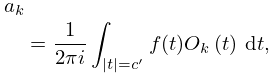
10.23.11 $$a_k=\frac{1}{2\pi \mathrm{i}}{\int }_{|t|=c^{\prime }}f(t)O_k\left(t\right)dt,$$ ,

ⓘ

Defines:

$a_k$ (locally)

Symbols:

$O_n\left(x\right)$: Neumann’s polynomial, $\pi$: the ratio of the circumference of a circle to its diameter, $dx$: differential of $x$ , $\mathrm{i}$: imaginary unit, $\int$: integral, $k$: nonnegative integer, $z$: complex variable and $f(t)$

A&S Ref:

9.1.83

Referenced by:

Erratum (V1.1.2) for Equation (10.23.11)

Permalink:

http://dlmf.nist.gov/10.23.E11

Encodings:

pMML, png, TeX

Errata (effective with 1.1.2):

Originally the contour of integration written incorrectly as $|z|=c^{\prime }$, has been corrected to be $|t|=c^{\prime }$.

Reported 2021-03-22 by Mark Dunster

See also:

Annotations for §10.23(iii), §10.23(iii), §10.23 and Ch.10

…

12: 3.5 Quadrature

§3.5 Quadrature

… ►

§3.5(iii) Romberg Integration

►Further refinements are achieved by Romberg integration. … ►For these cases the integration path may need to be deformed; see §3.5(ix). … ►

§3.5(ix) Other Contour Integrals

…

13: 35.2 Laplace Transform

… ►

35.2.1 $$g(𝐙)={\int }_{𝛀}\mathrm{etr}\left(-𝐙𝐗\right)f(𝐗)d𝐗,$$

ⓘ

Defines:

$g$: Laplace transformation of $f$ (locally)

Symbols:

$\mathrm{etr}\left(𝐀\right)$: exponential of trace, $\int$: integral, $𝐗$: real symmetric $m\times m$ matrix, $d$: differential of matrix, $𝛀$: space of positive-definite real symmetric $m\times m$ matrices, $𝐙$: complex symmetric $m\times m$ matrix and $f(𝐗)$: complex-valued function of matrix argument

Keywords:

Laplace transform

Referenced by:

§35.2

Permalink:

http://dlmf.nist.gov/35.2.E1

Encodings:

pMML, png, TeX

See also:

Annotations for §35.2, §35.2 and Ch.35

►where the integration variable $𝐗$ ranges over the space $𝛀$. … ►

35.2.3

ⓘ

Defines:

$\ast$: convolution operator (locally)

Symbols:

$\int$: integral, $𝐓$: real symmetric $m\times m$ matrix, $𝐗$: real symmetric $m\times m$ matrix, $d$: differential of matrix, : less-than for matrices, $f(𝐗)$: complex-valued function of matrix argument and $𝟎$: $m\times m$ matrix of zeros

Referenced by:

§35.6(ii)

Permalink:

http://dlmf.nist.gov/35.2.E3

Encodings:

pMML, png, TeX

See also:

Annotations for §35.2, §35.2 and Ch.35

14: 6.16 Mathematical Applications

… ►

6.16.2 $$S_n(x)=\sum _{k=0}^{n-1}\frac{\sin \left((2k+1)x\right)}{2k+1}=\frac{1}{2}{\int }_0^x\frac{\sin \left(2nt\right)}{\sin t}dt=\frac{1}{2}\mathrm{Si}\left(2nx\right)+R_n(x),$$

ⓘ

Defines:

$S_n(x)$: partial sum (locally)

Symbols:

$dx$: differential of $x$ , $\int$: integral, $\sin z$: sine function, $\mathrm{Si}\left(z\right)$: sine integral, $x$: real variable, $n$: nonnegative integer and $R_n(x)$: remainder term

Permalink:

http://dlmf.nist.gov/6.16.E2

Encodings:

pMML, png, TeX

See also:

Annotations for §6.16(i), §6.16 and Ch.6

… ►

6.16.3 $$R_n(x)=\frac{1}{2}{\int }_0^x\left(\frac{1}{\sin t}-\frac{1}{t}\right)\sin \left(2nt\right)dt.$$

ⓘ

Defines:

$R_n(x)$: remainder term (locally)

Symbols:

$dx$: differential of $x$ , $\int$: integral, $\sin z$: sine function, $x$: real variable and $n$: nonnegative integer

Permalink:

http://dlmf.nist.gov/6.16.E3

Encodings:

pMML, png, TeX

See also:

Annotations for §6.16(i), §6.16 and Ch.6

►By integration by parts …

15: 2.3 Integrals of a Real Variable

… ►

§2.3(i) Integration by Parts

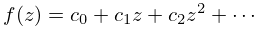
… ►Then the series obtained by substituting (2.3.7) into (2.3.1) and integrating formally term by term yields an asymptotic expansion: … ►derives from the neighborhood of the minimum of $p(t)$ in the integration range. … ►A uniform approximation can be constructed by quadratic change of integration variable: … ►We replace the limit $\kappa$ by $\mathrm{\infty }$ and integrate term-by-term: …

16: 1.14 Integral Transforms

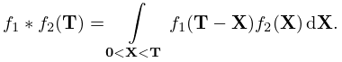
… ►In many applications $f(t)$ is absolutely integrable and $f^{\prime }(t)$ is continuous on $(-\mathrm{\infty },\mathrm{\infty })$. … ►Suppose $f(t)$ and $g(t)$ are absolutely and square integrable on $(-\mathrm{\infty },\mathrm{\infty })$, then … ►Suppose $f(t)$ and $g(t)$ are absolutely and square integrable on $[0,\mathrm{\infty })$, then … ►

Differentiation and Integration

… ►If $f(t)$ is absolutely integrable on $[0,R]$ for every finite $R$, and the integral (1.14.47) converges, then …

17: 30.4 Functions of the First Kind

… ►If $f(x)$ is mean-square integrable on $[-1,1]$, then formally … ►

30.4.8 $$c_n=(n+\frac{1}{2})\frac{(n-m)!}{(n+m)!}{\int }_{-1}^{1}f(t){\mathrm{𝖯𝗌}}_n^m(t,{\gamma }^2)dt.$$

ⓘ

Defines:

$c_n$: coefficient (locally)

Symbols:

$dx$: differential of $x$ , $!$: factorial (as in $n!$), $\int$: integral, ${\mathrm{𝖯𝗌}}_n^m(x,{\gamma }^2)$: spheroidal wave function of the first kind, $m$: nonnegative integer, $n\ge m$: integer degree, ${\gamma }^2$: real parameter and $f(x)$: function

Permalink:

http://dlmf.nist.gov/30.4.E8

Encodings:

pMML, png, TeX

See also:

Annotations for §30.4(iv), §30.4 and Ch.30

…

18: 8.21 Generalized Sine and Cosine Integrals

… ►(obtained from (5.2.1) by rotation of the integration path) is also needed. … ►In these representations the integration paths do not cross the negative real axis, and in the case of (8.21.4) and (8.21.5) the paths also exclude the origin. … ►

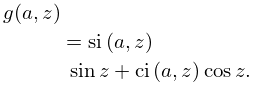
8.21.18 $$f(a,z)=\mathrm{si}(a,z)\cos z-\mathrm{ci}(a,z)\sin z,$$

ⓘ

Defines:

$f(a,z)$: auxiliary function (locally)

Symbols:

$\cos z$: cosine function, $\mathrm{ci}(a,z)$: generalized cosine integral, $\mathrm{si}(a,z)$: generalized sine integral, $\sin z$: sine function, $z$: complex variable and $a$: parameter

A&S Ref:

5.2.6 (This generalizes the form in AMS 55.)

Referenced by:

§8.21(vii)

Permalink:

http://dlmf.nist.gov/8.21.E18

Encodings:

pMML, png, TeX

See also:

Annotations for §8.21(vii), §8.21 and Ch.8

►

8.21.19 $$g(a,z)=\mathrm{si}(a,z)\sin z+\mathrm{ci}(a,z)\cos z.$$

ⓘ

Defines:

$g(a,z)$: auxiliary function (locally)

Symbols:

$\cos z$: cosine function, $\mathrm{ci}(a,z)$: generalized cosine integral, $\mathrm{si}(a,z)$: generalized sine integral, $\sin z$: sine function, $z$: complex variable and $a$: parameter

A&S Ref:

5.2.7 (This generalizes the form in AMS 55.)

Referenced by:

§8.21(vii)

Permalink:

http://dlmf.nist.gov/8.21.E19

Encodings:

pMML, png, TeX

See also:

Annotations for §8.21(vii), §8.21 and Ch.8

…

19: 21.7 Riemann Surfaces

… ►

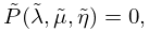
21.7.2 $$\tilde{P}(\tilde{\lambda },\tilde{\mu },\tilde{\eta })=0,$$

ⓘ

Defines:

$\tilde{P}(\tilde{\lambda },\tilde{\mu })$: polynomial (locally)

Permalink:

http://dlmf.nist.gov/21.7.E2

Encodings:

pMML, png, TeX

See also:

Annotations for §21.7(i), §21.7 and Ch.21

… ►If a local coordinate $z$ is chosen on the Riemann surface, then the local coordinate representation of these holomorphic differentials is given by …Note that for the purposes of integrating these holomorphic differentials, all cycles on the surface are a linear combination of the cycles $a_j$, $b_j$, $j=1,2,\mathrm{\dots },g$. … ►where $P_1$ and $P_2$ are points on $\mathrm{\Gamma }$, $𝝎=({\omega }_1,{\omega }_2,\mathrm{\dots },{\omega }_g)$, and the path of integration on $\mathrm{\Gamma }$ from $P_1$ to $P_2$ is identical for all components. … ►where again all integration paths are identical for all components. …

20: 3.11 Approximation Techniques

… ►

3.11.3 $$m_j={(-1)}^j{ϵ}_n(x_j),$$ $j=0,1,\mathrm{\dots },n+1$.

ⓘ

Defines:

$m_j$: approximation (locally)

Symbols:

${ϵ}_n(x)$: error

Permalink:

http://dlmf.nist.gov/3.11.E3

Encodings:

pMML, png, TeX

See also:

Annotations for §3.11(i), §3.11 and Ch.3

… ►The iterative process converges locally and quadratically (§3.8(i)). … ►They enjoy an orthogonal property with respect to integrals: … ►

3.11.16 $$R_{k,\mathrm{\ell }}(x)=\frac{p_0+p_{1}x+\mathrm{\cdots }+p_k{x}^k}{1+q_{1}x+\mathrm{\cdots }+q_{\mathrm{\ell }}{x}^{\mathrm{\ell }}}$$

ⓘ

Defines:

$R_{k,\mathrm{\ell }}(x)$: rational approximation (locally), $p_k$: coefficients (locally) and $q_{\mathrm{\ell }}$: coefficients (locally)

Referenced by:

§3.11(iii)

Permalink:

http://dlmf.nist.gov/3.11.E16

Encodings:

pMML, png, TeX

See also:

Annotations for §3.11(iii), §3.11 and Ch.3

… ►

3.11.20 $$f(z)=c_0+c_{1}z+c_2{z}^2+\mathrm{\cdots }$$

ⓘ

Defines:

$c_q$: coefficients (locally)

Referenced by:

§3.11(iv)

Permalink:

http://dlmf.nist.gov/3.11.E20

Encodings:

pMML, png, TeX

See also:

Annotations for §3.11(iv), §3.11 and Ch.3

…