locally integrable

SearchAdvancedHelp

(0.002 seconds)

1—10 of 39 matching pages

1: 2.6 Distributional Methods

… ►Let $f(t)$ be locally integrable on $[0,\mathrm{\infty })$. The Stieltjes transform of $f(t)$ is defined by …Since $f(t)$ is locally integrable on $[0,\mathrm{\infty })$, it defines a distribution by … ►In terms of the convolution product …of two locally integrable functions on $[0,\mathrm{\infty })$, (2.6.33) can be written …

2: 2.5 Mellin Transform Methods

… ►

§2.5(i) Introduction

►Let $f(t)$ be a locally integrable function on $(0,\mathrm{\infty })$, that is, ${\int }_{\rho }^{T}f(t)dt$ exists for all $\rho$ and $T$ satisfying . … ►Let $f(t)$ and $h(t)$ be locally integrable on $(0,\mathrm{\infty })$ and …Also, let … ►

2.5.24 $$h_2(t)=h(t)-h_1(t).$$

ⓘ

Symbols:

$h(x)$: locally integrable function

Referenced by:

§2.5(iii)

Permalink:

http://dlmf.nist.gov/2.5.E24

Encodings:

pMML, png, TeX

See also:

Annotations for §2.5(ii), §2.5 and Ch.2

…

3: 1.16 Distributions

… ►A distribution $\mathrm{\Lambda }$ is called regular if there is a locally integrable function $f$ on $I$ (i. … ►If $f$ is a locally integrable function then its distributional derivative is $𝐷f={\mathrm{\Lambda }}_f^{\prime }$. … ►A locally integrable function $f(x)=f(x_1,x_2,\mathrm{\dots },x_n)$ gives rise to a distribution ${\mathrm{\Lambda }}_f$ defined by …

4: 9.13 Generalized Airy Functions

… ►

9.13.25 $$A_k(z,p)=\frac{1}{2\pi \mathrm{i}}{\int }_{{ℒ}_k}{t}^{-p}\exp \left(zt-\frac{1}{3}{t}^3\right)dt,$$ $k=1,2,3$, $p\in ℂ$,

ⓘ

Defines:

$k$: index (locally) and $p$: parameter (locally)

Symbols:

$A_k(z,p)$: generalized Airy function, $\pi$: the ratio of the circumference of a circle to its diameter, $ℂ$: complex plane, $dx$: differential of $x$ , $\in$: element of, $\exp z$: exponential function, $\mathrm{i}$: imaginary unit, $\int$: integral, $z$: complex variable and $ℒ$: integration path

Sources:

Reid (1972, (A4), p. 362); Drazin and Reid (1981, (A4), p. 466)

Referenced by:

§9.13(ii)

Permalink:

http://dlmf.nist.gov/9.13.E25

Encodings:

pMML, png, TeX

See also:

Annotations for §9.13(ii), §9.13 and Ch.9

…

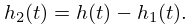
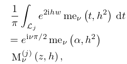
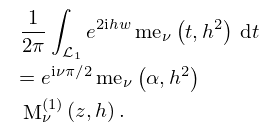
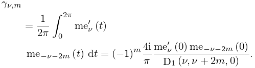
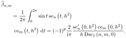
5: 28.28 Integrals, Integral Representations, and Integral Equations

… ►In (28.28.7)–(28.28.9) the paths of integration ${ℒ}_j$ are given by … ►

28.28.7 $$\frac{1}{\pi }{\int }_{{ℒ}_j}{\mathrm{e}}^{2\mathrm{i}hw}{\mathrm{me}}_{\nu }(t,h^2)dt={\mathrm{e}}^{\mathrm{i}\nu \pi /2}{\mathrm{me}}_{\nu }(\alpha ,h^2){\mathrm{M}}_{\nu }^{(j)}(z,h),$$ $j=3,4$,

ⓘ

Symbols:

${\mathrm{me}}_n(z,q)$: Mathieu function, $\pi$: the ratio of the circumference of a circle to its diameter, $dx$: differential of $x$ , $\mathrm{e}$: base of natural logarithm, $\mathrm{i}$: imaginary unit, $\int$: integral, ${\mathrm{M}}_{\nu }^{(j)}(z,h)$: modified Mathieu function, $h$: parameter, $j$: integer, $z$: complex variable, $\nu$: complex parameter, $w(z)$: Mathieu’s equation solution, $\alpha$: parameter and ${ℒ}_j$: integration paths

A&S Ref:

20.7.18 (in slightly different notation)

Referenced by:

§28.28(i)

Permalink:

http://dlmf.nist.gov/28.28.E7

Encodings:

pMML, png, TeX

See also:

Annotations for §28.28(i), §28.28 and Ch.28

… ►

28.28.9 $$\frac{1}{2\pi }{\int }_{{ℒ}_1}{\mathrm{e}}^{2\mathrm{i}hw}{\mathrm{me}}_{\nu }(t,h^2)dt={\mathrm{e}}^{\mathrm{i}\nu \pi /2}{\mathrm{me}}_{\nu }(\alpha ,h^2){\mathrm{M}}_{\nu }^{(1)}(z,h).$$

ⓘ

Symbols:

${\mathrm{me}}_n(z,q)$: Mathieu function, $\pi$: the ratio of the circumference of a circle to its diameter, $dx$: differential of $x$ , $\mathrm{e}$: base of natural logarithm, $\mathrm{i}$: imaginary unit, $\int$: integral, ${\mathrm{M}}_{\nu }^{(j)}(z,h)$: modified Mathieu function, $h$: parameter, $z$: complex variable, $\nu$: complex parameter, $w(z)$: Mathieu’s equation solution, $\alpha$: parameter and ${ℒ}_j$: integration paths

Referenced by:

§28.28(i)

Permalink:

http://dlmf.nist.gov/28.28.E9

Encodings:

pMML, png, TeX

See also:

Annotations for §28.28(i), §28.28 and Ch.28

… ►

28.28.33 $${\gamma }_{\nu ,m}=\frac{1}{2\pi }{\int }_0^{2\pi }{\mathrm{me}}_{\nu }^{\prime }\left(t\right){\mathrm{me}}_{-\nu -2m}\left(t\right)dt={(-1)}^m\frac{4\mathrm{i}}{\pi }\frac{{\mathrm{me}}_{\nu }^{\prime }\left(0\right){\mathrm{me}}_{-\nu -2m}\left(0\right)}{{\mathrm{D}}_1(\nu ,\nu +2m,0)}.$$

ⓘ

Defines:

${\gamma }_{\nu ,m}$ (locally)

Symbols:

${\mathrm{D}}_j(\nu ,\mu ,z)$: cross-products of modified Mathieu functions and their derivatives, ${\mathrm{me}}_n(z,q)$: Mathieu function, $\pi$: the ratio of the circumference of a circle to its diameter, $dx$: differential of $x$ , $\mathrm{i}$: imaginary unit, $\int$: integral, $m$: integer, $h$: parameter and $\nu$: complex parameter

Permalink:

http://dlmf.nist.gov/28.28.E33

Encodings:

pMML, png, TeX

See also:

Annotations for §28.28(iii), §28.28 and Ch.28

… ►

28.28.43 $${\widehat{\beta }}_{n,m}=\frac{1}{2\pi }{\int }_0^{2\pi }\sin t{\mathrm{se}}_n(t,h^2){\mathrm{ce}}_m(t,h^2)dt={(-1)}^p\frac{2}{\mathrm{i}\pi }\frac{{\mathrm{se}}_n^{\prime }(0,h^2){\mathrm{ce}}_m(0,h^2)}{h{\mathrm{Dsc}}_1(n,m,0)}.$$

ⓘ

Defines:

${\widehat{\beta }}_{n,m}$ (locally)

Symbols:

${\mathrm{Dsc}}_j(n,m,z)$: cross-products of radial Mathieu functions and their derivatives, ${\mathrm{ce}}_n(z,q)$: Mathieu function, ${\mathrm{se}}_n(z,q)$: Mathieu function, $\pi$: the ratio of the circumference of a circle to its diameter, $dx$: differential of $x$ , $\mathrm{i}$: imaginary unit, $\int$: integral, $\sin z$: sine function, $m$: integer, $h$: parameter and $n$: integer

Permalink:

http://dlmf.nist.gov/28.28.E43

Encodings:

pMML, png, TeX

See also:

Annotations for §28.28(iv), §28.28 and Ch.28

…

6: 1.18 Linear Second Order Differential Operators and Eigenfunction Expansions

… ►Thus, and this is a case where $q(x)$ is not continuous, if $q(x)=-\alpha \delta \left(x-a\right)$, $\alpha >0$, there will be an $L^2$ eigenfunction localized in the vicinity of $x=a$, with a negative eigenvalue, thus disjoint from the continuous spectrum on $[0,\mathrm{\infty })$. …

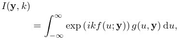
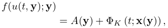
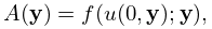
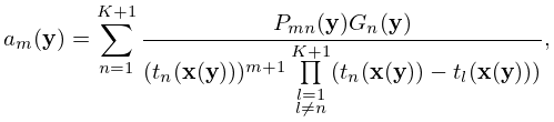
7: 36.12 Uniform Approximation of Integrals

… ►In the cuspoid case (one integration variable) ►

36.12.1 $$I(𝐲,k)={\int }_{-\mathrm{\infty }}^{\mathrm{\infty }}\exp \left(\mathrm{i}kf(u;𝐲)\right)g(u,𝐲)du,$$

ⓘ

Defines:

$I(𝐲,k)$: oscillatory integral (locally)

Symbols:

$dx$: differential of $x$ , $\exp z$: exponential function, $\mathrm{i}$: imaginary unit, $\int$: integral, $k$: variable, $g(u,𝐲)$: function, $f(u,𝐲)$: function and $u(t;𝐲)$: mapping

Referenced by:

§36.13

Permalink:

http://dlmf.nist.gov/36.12.E1

Encodings:

pMML, png, TeX

See also:

Annotations for §36.12(i), §36.12 and Ch.36

… ►

36.12.4 $$f(u(t,𝐲);𝐲)=A(𝐲)+{\mathrm{\Phi }}_K(t;𝐱(𝐲)),$$

ⓘ

Defines:

$u(t;𝐲)$: mapping (locally)

Symbols:

${\mathrm{\Phi }}_K(t;𝐱)$: cuspoid catastrophe of codimension $K$ , $t$: variable, $K$: codimension, $f(u,𝐲)$: function, $𝐱(𝐲)$: function and $A(𝐲)$: function

Permalink:

http://dlmf.nist.gov/36.12.E4

Encodings:

pMML, png, TeX

See also:

Annotations for §36.12(i), §36.12 and Ch.36

… ►

36.12.6 $$A(𝐲)=f(u(0,𝐲);𝐲),$$

ⓘ

Defines:

$A(𝐲)$: function (locally)

Symbols:

$f(u,𝐲)$: function and $u(t;𝐲)$: mapping

Permalink:

http://dlmf.nist.gov/36.12.E6

Encodings:

pMML, png, TeX

See also:

Annotations for §36.12(i), §36.12 and Ch.36

… ►

36.12.8 $$a_m(𝐲)=\sum _{n=1}^{K+1}\frac{P_{mn}(𝐲)G_n(𝐲)}{{(t_n(𝐱(𝐲)))}^{m+1}\prod _{\begin{array}{c}l=1\\ l\ne n\end{array}}^{K+1}(t_n(𝐱(𝐲))-t_l(𝐱(𝐲)))},$$

ⓘ

Defines:

$a_m(𝐲)$: function (locally)

Symbols:

$l$: integer, $n$: integer, $m$: integer, $K$: codimension, $𝐱(𝐲)$: function and $t_j(𝐱)$: solutions

Permalink:

http://dlmf.nist.gov/36.12.E8

Encodings:

pMML, png, TeX

See also:

Annotations for §36.12(i), §36.12 and Ch.36

…

8: 32.2 Differential Equations

… ►be a nonlinear second-order differential equation in which $F$ is a rational function of $w$ and $dw/dz$, and is locally analytic in $z$, that is, analytic except for isolated singularities in $ℂ$. In general the singularities of the solutions are movable in the sense that their location depends on the constants of integration associated with the initial or boundary conditions. … ►in which $a(z)$, $b(z)$, $c(z)$, $d(z)$, and $\varphi (z)$ are locally analytic functions. …

9: 31.9 Orthogonality

… ►The integration path begins at $z=\zeta$, encircles $z=1$ once in the positive sense, followed by $z=0$ once in the positive sense, and so on, returning finally to $z=\zeta$. The integration path is called a Pochhammer double-loop contour (compare Figure 5.12.3). … ►

$$f_0(q_m,z)=H\mathrm{\ell }(a,q_m;\alpha ,\beta ,\gamma ,\delta ;z),$$

►

$$f_1(q_m,z)=H\mathrm{\ell }(1-a,\alpha \beta -q_m;\alpha ,\beta ,\delta ,\gamma ;1-z),$$

… ►and the integration paths ${ℒ}_1$, ${ℒ}_2$ are Pochhammer double-loop contours encircling distinct pairs of singularities $\{0,1\}$, $\{0,a\}$, $\{1,a\}$. …

10: 15.9 Relations to Other Functions

… ►where the contour of integration is located to the right of the poles of the gamma functions in the integrand, and ►

15.9.14 $${\mathrm{\Phi }}_{\lambda }^{(\alpha ,\beta )}(t)={(2\cosh t)}^{\mathrm{i}\lambda -\alpha -\beta -1}F(\genfrac{}{}{0pt}{}{\frac{1}{2}(\alpha +\beta +1-\mathrm{i}\lambda ),\frac{1}{2}(\alpha -\beta +1-\mathrm{i}\lambda )}{1-\mathrm{i}\lambda };{\mathrm{sech}}^{2}t).$$

ⓘ

Defines:

${\mathrm{\Phi }}_{\lambda }^{(\alpha ,\beta )}(t)$: function (locally)

Symbols:

$F(a,b;c;z)$ or $F(\genfrac{}{}{0pt}{}{a,b}{c};z)$: $={}_2{}^{}F_1^{}(a,b;c;z)$ Gauss’ hypergeometric function, $\cosh z$: hyperbolic cosine function, $\mathrm{sech}z$: hyperbolic secant function, $\mathrm{i}$: imaginary unit and $(a,b)$: open interval

Permalink:

http://dlmf.nist.gov/15.9.E14

Encodings:

pMML, png, TeX

See also:

Annotations for §15.9(ii), §15.9 and Ch.15

…