locally%20integrable

SearchAdvancedHelp

(0.002 seconds)

1—10 of 358 matching pages

1: 6.16 Mathematical Applications

… ►

6.16.2 $$S_n(x)=\sum _{k=0}^{n-1}\frac{\sin \left((2k+1)x\right)}{2k+1}=\frac{1}{2}{\int }_0^x\frac{\sin \left(2nt\right)}{\sin t}dt=\frac{1}{2}\mathrm{Si}\left(2nx\right)+R_n(x),$$

ⓘ

Defines:

$S_n(x)$: partial sum (locally)

Symbols:

$dx$: differential of $x$ , $\int$: integral, $\sin z$: sine function, $\mathrm{Si}\left(z\right)$: sine integral, $x$: real variable, $n$: nonnegative integer and $R_n(x)$: remainder term

Permalink:

http://dlmf.nist.gov/6.16.E2

Encodings:

pMML, png, TeX

See also:

Annotations for §6.16(i), §6.16 and Ch.6

… ►

6.16.3 $$R_n(x)=\frac{1}{2}{\int }_0^x\left(\frac{1}{\sin t}-\frac{1}{t}\right)\sin \left(2nt\right)dt.$$

ⓘ

Defines:

$R_n(x)$: remainder term (locally)

Symbols:

$dx$: differential of $x$ , $\int$: integral, $\sin z$: sine function, $x$: real variable and $n$: nonnegative integer

Permalink:

http://dlmf.nist.gov/6.16.E3

Encodings:

pMML, png, TeX

See also:

Annotations for §6.16(i), §6.16 and Ch.6

►By integration by parts … ►

►►

Figure 6.16.2: The logarithmic integral $\mathrm{li}\left(x\right)$, together with vertical bars indicating the value of $\pi (x)$ for $x=10,20,\mathrm{\dots },1000$. Magnify

2: 25.12 Polylogarithms

… ►

25.12.9 $$\sum _{n=1}^{\mathrm{\infty }}\frac{\sin \left(n\theta \right)}{n^2}=-{\int }_0^{\theta }\ln \left(2\sin \left(\frac{1}{2}x\right)\right)dx.$$

ⓘ

Symbols:

$dx$: differential of $x$ , $\int$: integral, $\ln z$: principal branch of logarithm function, $\sin z$: sine function, $n$: nonnegative integer, $x$: real variable and $\theta$: phase

Keywords:

definite integral, infinite series

Source:

Maximon (2003, (8.7), (8.8), p. 2813)

A&S Ref:

27.8.6 (integration of first series)

Referenced by:

1st item

Permalink:

http://dlmf.nist.gov/25.12.E9

Encodings:

pMML, png, TeX

See also:

Annotations for §25.12(i), §25.12 and Ch.25

… ►

►►

Figure 25.12.1: Dilogarithm function ${\mathrm{Li}}_2\left(x\right)$, Magnify

►

►

►

Figure 25.12.2: Absolute value of the dilogarithm function $\left|{\mathrm{Li}}_2\left(x+\mathrm{i}y\right)\right|$, $-20\le x\le 20$, $-20\le y\le 20$. … Magnify 3D Help

… ►

25.12.14 $$F_s(x)=\frac{1}{\mathrm{\Gamma }\left(s+1\right)}{\int }_0^{\mathrm{\infty }}\frac{t^s}{{\mathrm{e}}^{t-x}+1}dt,$$ $s>-1$,

ⓘ

Defines:

$F_s(x)$: Fermi–Dirac integral (locally)

Symbols:

$\mathrm{\Gamma }\left(z\right)$: gamma function, $dx$: differential of $x$ , $\mathrm{e}$: base of natural logarithm, $\int$: integral, $x$: real variable and $s$: complex variable

Keywords:

definition, Fermi–Dirac integral, improper integral, integral representation

Source:

Dingle (1957b, (1), p. 226)

Referenced by:

(25.12.16), 3rd item, 5th item

Permalink:

http://dlmf.nist.gov/25.12.E14

Encodings:

pMML, png, TeX

See also:

Annotations for §25.12(iii), §25.12 and Ch.25

►

25.12.15 $$G_s(x)=\frac{1}{\mathrm{\Gamma }\left(s+1\right)}{\int }_0^{\mathrm{\infty }}\frac{t^s}{{\mathrm{e}}^{t-x}-1}dt,$$ $s>-1$, ; or $s>0$, $x\le 0$,

ⓘ

Defines:

$G_s(x)$: Bose–Einstein integral (locally)

Symbols:

$\mathrm{\Gamma }\left(z\right)$: gamma function, $dx$: differential of $x$ , $\mathrm{e}$: base of natural logarithm, $\int$: integral, $x$: real variable and $s$: complex variable

Keywords:

Bose–Einstein integral, definition, improper integral, integral representation

Source:

Dingle (1957a, p. 240)

Referenced by:

(25.12.16)

Permalink:

http://dlmf.nist.gov/25.12.E15

Encodings:

pMML, png, TeX

See also:

Annotations for §25.12(iii), §25.12 and Ch.25

…

3: 31.9 Orthogonality

… ►The integration path begins at $z=\zeta$, encircles $z=1$ once in the positive sense, followed by $z=0$ once in the positive sense, and so on, returning finally to $z=\zeta$. The integration path is called a Pochhammer double-loop contour (compare Figure 5.12.3). … ►

$$f_0(q_m,z)=H\mathrm{\ell }(a,q_m;\alpha ,\beta ,\gamma ,\delta ;z),$$

►

$$f_1(q_m,z)=H\mathrm{\ell }(1-a,\alpha \beta -q_m;\alpha ,\beta ,\delta ,\gamma ;1-z),$$

… ►and the integration paths ${ℒ}_1$, ${ℒ}_2$ are Pochhammer double-loop contours encircling distinct pairs of singularities $\{0,1\}$, $\{0,a\}$, $\{1,a\}$. …

4: 2.6 Distributional Methods

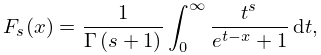
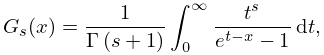
… ►Let $f(t)$ be locally integrable on $[0,\mathrm{\infty })$. The Stieltjes transform of $f(t)$ is defined by …Since $f(t)$ is locally integrable on $[0,\mathrm{\infty })$, it defines a distribution by … ►In terms of the convolution product …of two locally integrable functions on $[0,\mathrm{\infty })$, (2.6.33) can be written …

5: 2.5 Mellin Transform Methods

… ►

§2.5(i) Introduction

►Let $f(t)$ be a locally integrable function on $(0,\mathrm{\infty })$, that is, ${\int }_{\rho }^{T}f(t)dt$ exists for all $\rho$ and $T$ satisfying . … ►We now apply (2.5.5) with , and then translate the integration contour to the right. … ►Let $f(t)$ and $h(t)$ be locally integrable on $(0,\mathrm{\infty })$ and …Also, let …

6: Bibliography V

… ►

Integrating products of Bessel functions with an additional exponential or rational factor. Comput. Phys. Comm. 178 (8), pp. 578–590.

ⓘ

Notes:

Associated computer program available online

External Links:

ISSN 0010-4655, Document, FullText, MathReview Entry, ZentralBlatt

Referenced by:

§10.74(vii), §10.74(vii).

Encodings:

BibTeX

… ►

Error estimates for Rayleigh-Ritz approximations of eigenvalues and eigenfunctions of the Mathieu and spheroidal wave equation. Constr. Approx. 20 (1), pp. 39–54.

ⓘ

External Links:

ISSN 0176-4276, Document, MathReview, ZentralBlatt

Referenced by:

§30.16(i), §30.16(ii), §30.16(ii).

Encodings:

BibTeX

… ►

On the localization and computation of zeros of Bessel functions. Z. Angew. Math. Mech. 77 (6), pp. 467–475.

ⓘ

External Links:

ISSN 0044-2267, Document, MathReview, ZentralBlatt

Referenced by:

§10.74(vi).

Encodings:

BibTeX

… ►

The topological degree theory for the localization and computation of complex zeros of Bessel functions. Numer. Funct. Anal. Optim. 18 (1-2), pp. 227–234.

ⓘ

External Links:

ISSN 0163-0563, Document, MathReview, ZentralBlatt

Referenced by:

§10.74(vi).

Encodings:

BibTeX

7: Bibliography C

… ►

Orthogonalization Procedures and the Localization of Wannier Functions. Phys. Rev. 105, pp. 102–103.

ⓘ

External Links:

Document, Link, ZentralBlatt

Referenced by:

Profile Bille C. Carlson.

Encodings:

BibTeX

… ►

Elliptic Integrals: Symmetry and Symbolic Integration. In Tricomi’s Ideas and Contemporary Applied Mathematics (Rome/Turin, 1997), Atti dei Convegni Lincei, Vol. 147, pp. 161–181.

ⓘ

External Links:

MathReview (S. L. Kalla), ZentralBlatt

Referenced by:

§19.26(iii), §19.29(i).

Encodings:

BibTeX

… ►

Numerical integration of related Hankel transforms by quadrature and continued fraction expansion. Geophysics 48 (12), pp. 1671–1686.

ⓘ

Notes:

Fortran code.

External Links:

ISSN 0098-3500, Document

Referenced by:

§10.77(ix).

Encodings:

BibTeX

… ►

A method for numerical integration on an automatic copmputer. Numer. Math. 2 (4), pp. 197–205.

ⓘ

External Links:

ISSN 0029-599X, Document, MathReview (A. H. Stroud), ZentralBlatt

Referenced by:

§3.5(iv).

Encodings:

BibTeX

… ►

On the integration of incomplete elliptic integrals. Proc. Roy. Soc. London Ser. A 444, pp. 525–532.

ⓘ

External Links:

ISSN 0962-8444, FullText, MathReview, ZentralBlatt

Referenced by:

§19.13(i), §19.13(ii).

Encodings:

BibTeX

…

8: 3.8 Nonlinear Equations

… ► … ►If $\zeta$ is a simple zero, then the iteration converges locally and quadratically. … ►It converges locally and quadratically for both $ℝ$ and $ℂ$. … ►The method converges locally and quadratically, except when the wanted quadratic factor is a multiple factor of $q(z)$. … ►The rule converges locally and is cubically convergent. …

9: 31.3 Basic Solutions

… ► $H\mathrm{\ell }(a,q;\alpha ,\beta ,\gamma ,\delta ;z)$ denotes the solution of (31.2.1) that corresponds to the exponent $0$ at $z=0$ and assumes the value $1$ there. If the other exponent is not a positive integer, that is, if $\gamma \ne 0,-1,-2,\mathrm{\dots }$, then from §2.7(i) it follows that $H\mathrm{\ell }(a,q;\alpha ,\beta ,\gamma ,\delta ;z)$ exists, is analytic in the disk , and has the Maclaurin expansion … ►Solutions (31.3.1) and (31.3.5)–(31.3.11) comprise a set of 8 local solutions of (31.2.1): 2 per singular point. …For example, $H\mathrm{\ell }(a,q;\alpha ,\beta ,\gamma ,\delta ;z)$ is equal to … ►The full set of 192 local solutions of (31.2.1), equivalent in 8 sets of 24, resembles Kummer’s set of 24 local solutions of the hypergeometric equation, which are equivalent in 4 sets of 6 solutions (§15.10(ii)); see Maier (2007).

10: 20 Theta Functions

Chapter 20 Theta Functions

…