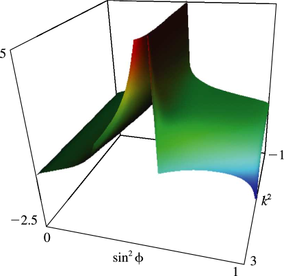
About the Project

lemniscate%20constants

AdvancedHelp

(0.002 seconds)

1—10 of 498 matching pages

1: 22.18 Mathematical Applications
Lemniscate
In polar coordinates, x = r cos ϕ , y = r sin ϕ , the lemniscate is given by r 2 = cos ( 2 ϕ ) , 0 ϕ 2 π . …
22.18.7 a x 2 y 2 + b ( x 2 y + x y 2 ) + c ( x 2 + y 2 ) + 2 d x y + e ( x + y ) + f = 0 ,
in which a , b , c , d , e , f are real constants, can be achieved in terms of single-valued functions. …
2: 19.20 Special Cases
R F ( 0 , 0 , z ) = .
The first lemniscate constant is given by
19.20.2 0 1 d t 1 t 4 = R F ( 0 , 1 , 2 ) = ( Γ ( 1 4 ) ) 2 4 ( 2 π ) 1 / 2 = 1.31102 87771 46059 90523 .
19.20.21 R D ( x , x , z ) = 3 z x ( R C ( z , x ) 1 z ) , x z , x z 0 .
The second lemniscate constant is given by …
3: 19.30 Lengths of Plane Curves
§19.30(iii) Bernoulli’s Lemniscate
For 0 θ 1 4 π , the arclength s of Bernoulli’s lemniscate …The perimeter length P of the lemniscate is given by …
4: Bibliography T
  • J. Todd (1975) The lemniscate constants. Comm. ACM 18 (1), pp. 14–19.
  • 5: 8.26 Tables
  • Khamis (1965) tabulates P ( a , x ) for a = 0.05 ( .05 ) 10 ( .1 ) 20 ( .25 ) 70 , 0.0001 x 250 to 10D.

  • Zhang and Jin (1996, Table 3.8) tabulates γ ( a , x ) for a = 0.5 , 1 , 3 , 5 , 10 , 25 , 50 , 100 , x = 0 ( .1 ) 1 ( 1 ) 3 , 5 ( 5 ) 30 , 50 , 100 to 8D or 8S.

  • Abramowitz and Stegun (1964, pp. 245–248) tabulates E n ( x ) for n = 2 , 3 , 4 , 10 , 20 , x = 0 ( .01 ) 2 to 7D; also ( x + n ) e x E n ( x ) for n = 2 , 3 , 4 , 10 , 20 , x 1 = 0 ( .01 ) 0.1 ( .05 ) 0.5 to 6S.

  • Pagurova (1961) tabulates E n ( x ) for n = 0 ( 1 ) 20 , x = 0 ( .01 ) 2 ( .1 ) 10 to 4-9S; e x E n ( x ) for n = 2 ( 1 ) 10 , x = 10 ( .1 ) 20 to 7D; e x E p ( x ) for p = 0 ( .1 ) 1 , x = 0.01 ( .01 ) 7 ( .05 ) 12 ( .1 ) 20 to 7S or 7D.

  • Zhang and Jin (1996, Table 19.1) tabulates E n ( x ) for n = 1 , 2 , 3 , 5 , 10 , 15 , 20 , x = 0 ( .1 ) 1 , 1.5 , 2 , 3 , 5 , 10 , 20 , 30 , 50 , 100 to 7D or 8S.

  • 6: 20 Theta Functions
    Chapter 20 Theta Functions
    7: 19.3 Graphics
    See accompanying text
    Figure 19.3.6: Π ( ϕ , 2 , k ) as a function of k 2 and sin 2 ϕ for 1 k 2 3 , 0 sin 2 ϕ < 1 . …Its value tends to as k 2 1 + by (19.6.6), and to the negative of the second lemniscate constant (see (19.20.22)) as k 2 ( = csc 2 ϕ ) 2 . Magnify 3D Help
    8: 19.21 Connection Formulas
    The case z = 1 shows that the product of the two lemniscate constants, (19.20.2) and (19.20.22), is π / 4 . …
    9: 5.22 Tables
    Abramowitz and Stegun (1964, Chapter 6) tabulates Γ ( x ) , ln Γ ( x ) , ψ ( x ) , and ψ ( x ) for x = 1 ( .005 ) 2 to 10D; ψ ′′ ( x ) and ψ ( 3 ) ( x ) for x = 1 ( .01 ) 2 to 10D; Γ ( n ) , 1 / Γ ( n ) , Γ ( n + 1 2 ) , ψ ( n ) , log 10 Γ ( n ) , log 10 Γ ( n + 1 3 ) , log 10 Γ ( n + 1 2 ) , and log 10 Γ ( n + 2 3 ) for n = 1 ( 1 ) 101 to 8–11S; Γ ( n + 1 ) for n = 100 ( 100 ) 1000 to 20S. Zhang and Jin (1996, pp. 67–69 and 72) tabulates Γ ( x ) , 1 / Γ ( x ) , Γ ( x ) , ln Γ ( x ) , ψ ( x ) , ψ ( x ) , ψ ( x ) , and ψ ( x ) for x = 0 ( .1 ) 5 to 8D or 8S; Γ ( n + 1 ) for n = 0 ( 1 ) 100 ( 10 ) 250 ( 50 ) 500 ( 100 ) 3000 to 51S. … Abramov (1960) tabulates ln Γ ( x + i y ) for x = 1 ( .01 ) 2 , y = 0 ( .01 ) 4 to 6D. Abramowitz and Stegun (1964, Chapter 6) tabulates ln Γ ( x + i y ) for x = 1 ( .1 ) 2 , y = 0 ( .1 ) 10 to 12D. …Zhang and Jin (1996, pp. 70, 71, and 73) tabulates the real and imaginary parts of Γ ( x + i y ) , ln Γ ( x + i y ) , and ψ ( x + i y ) for x = 0.5 , 1 , 5 , 10 , y = 0 ( .5 ) 10 to 8S.
    10: 25.12 Polylogarithms
    See accompanying text
    Figure 25.12.1: Dilogarithm function Li 2 ( x ) , 20 x < 1 . Magnify
    See accompanying text
    Figure 25.12.2: Absolute value of the dilogarithm function | Li 2 ( x + i y ) | , 20 x 20 , 20 y 20 . … Magnify 3D Help
    25.12.11 Li s ( z ) z Γ ( s ) 0 x s 1 e x z d x ,
    25.12.14 F s ( x ) = 1 Γ ( s + 1 ) 0 t s e t x + 1 d t , s > 1 ,
    Sometimes the factor 1 / Γ ( s + 1 ) is omitted. …