large variable and%2For large parameter

SearchAdvancedHelp

(0.011 seconds)

21—30 of 73 matching pages

21: Bibliography L

… ►

The solutions of the Mathieu equation with a complex variable and at least one parameter large. Trans. Amer. Math. Soc. 36 (3), pp. 637–695.

ⓘ

External Links:

ISSN 0002-9947, FullText, MathReview Entry, ZentralBlatt

Referenced by:

§28.8(iv).

Encodings:

BibTeX

… ►

A Numerical Library in Java for Scientists & Engineers. Chapman & Hall/CRC, Boca Raton, FL.

ⓘ

Notes:

With 1 CD-ROM (Windows, Macintosh and Unix) containing a large general purpose mathematical software collection written in Java including a collection of special function classes. The functions are computed for real variables only. (See Lau (1995) for C version).

External Links:

ISBN 1-58488-430-4, MathReview Entry, ZentralBlatt

Referenced by:

H. T. Lau (1995).

Encodings:

BibTeX

… ►

Asymptotics of the first Appell function $F_1$ with large parameters II. Integral Transforms Spec. Funct. 24 (12), pp. 982–999.

ⓘ

External Links:

ISSN 1065-2469, Document, FullText, MathReview Entry, ZentralBlatt

Referenced by:

§16.13, §16.13.

Encodings:

BibTeX

►

Asymptotics of the first Appell function $F_1$ with large parameters. Integral Transforms Spec. Funct. 24 (9), pp. 715–733.

ⓘ

External Links:

ISSN 1065-2469, Document, FullText, MathReview Entry, ZentralBlatt

Referenced by:

§16.13, §16.13.

Encodings:

BibTeX

… ►

Asymptotic expansions of the Whittaker functions for large order parameter. Methods Appl. Anal. 6 (2), pp. 249–256.

ⓘ

Notes:

Dedicated to Richard A. Askey on the occasion of his 65th birthday, Part II

External Links:

ISSN 1073-2772, Pdf, MathReview, ZentralBlatt

Referenced by:

§13.21(i), §13.24(ii).

Encodings:

BibTeX

…

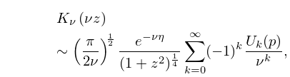
22: 10.41 Asymptotic Expansions for Large Order

… ►

10.41.4 $$K_{\nu }\left(\nu z\right)\sim {\left(\frac{\pi }{2\nu }\right)}^{\frac{1}{2}}\frac{{\mathrm{e}}^{-\nu \eta }}{{(1+z^2)}^{\frac{1}{4}}}\sum _{k=0}^{\mathrm{\infty }}{(-1)}^k\frac{U_k(p)}{{\nu }^k},$$

ⓘ

Symbols:

$\sim$: Poincaré asymptotic expansion, $\pi$: the ratio of the circumference of a circle to its diameter, $\mathrm{e}$: base of natural logarithm, $K_{\nu }\left(z\right)$: modified Bessel function of the second kind, $k$: nonnegative integer, $z$: complex variable, $\nu$: complex parameter, $\eta$ and $U_k(p)$: polynomial coefficient

A&S Ref:

9.7.8

Permalink:

http://dlmf.nist.gov/10.41.E4

Encodings:

pMML, png, TeX

See also:

Annotations for §10.41(ii), §10.41 and Ch.10

…

23: Bibliography O

… ►

Uniform asymptotic expansions for hypergeometric functions with large parameters. I. Analysis and Applications (Singapore) 1 (1), pp. 111–120.

ⓘ

External Links:

ISSN 0219-5305, Document, MathReview, ZentralBlatt

Referenced by:

§15.12(iii).

Encodings:

BibTeX

►

Uniform asymptotic expansions for hypergeometric functions with large parameters. II. Analysis and Applications (Singapore) 1 (1), pp. 121–128.

ⓘ

External Links:

ISSN 0219-5305, Document, MathReview, ZentralBlatt

Referenced by:

§15.12(iii).

Encodings:

BibTeX

… ►

Uniform asymptotic expansions for hypergeometric functions with large parameters. III. Analysis and Applications (Singapore) 8 (2), pp. 199–210.

ⓘ

External Links:

ISSN 0219-5305, Document, MathReview (Javier Segura), ZentralBlatt

Referenced by:

§15.12(iii).

Encodings:

BibTeX

… ►

Legendre functions with both parameters large. Philos. Trans. Roy. Soc. London Ser. A 278, pp. 175–185.

ⓘ

External Links:

FullText, MathReview (P. F. Hsieh), ZentralBlatt

Referenced by:

§14.15(v), §14.15(v).

Encodings:

BibTeX

… ►

Whittaker functions with both parameters large: Uniform approximations in terms of parabolic cylinder functions. Proc. Roy. Soc. Edinburgh Sect. A 86 (3-4), pp. 213–234.

ⓘ

External Links:

ISSN 0308-2105, MathReview (P. F. Hsieh), ZentralBlatt

Referenced by:

§13.20(iii), §13.20(iv).

Encodings:

BibTeX

…

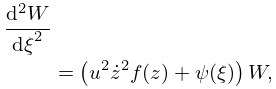
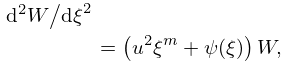
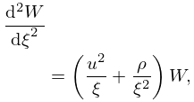
24: 2.8 Differential Equations with a Parameter

… ►

2.8.3 $$\frac{d^{2}W}{{d\xi }^2}=\left(u^2{\dot{z}}^{2}f(z)+\psi (\xi )\right)W,$$

ⓘ

Symbols:

$\frac{df}{dx}$: derivative of $f$ with respect to $x$ , $f(x)$: function, $u$: large real or complex parameter, $W$: change of variable, $\dot{z}$: derivative of $z$ with respect to $\xi$ and $\psi (\xi )$: function

Permalink:

http://dlmf.nist.gov/2.8.E3

Encodings:

pMML, png, TeX

See also:

Annotations for §2.8(i), §2.8 and Ch.2

… ►

2.8.8 $$d^{2}W/{d\xi }^2=\left(u^2{\xi }^m+\psi (\xi )\right)W,$$

ⓘ

Symbols:

$\frac{df}{dx}$: derivative of $f$ with respect to $x$ , $u$: large real or complex parameter, $W$: change of variable and $\psi (\xi )$: function

Referenced by:

§2.8(i), §2.8(iv)

Permalink:

http://dlmf.nist.gov/2.8.E8

Encodings:

pMML, png, TeX

See also:

Annotations for §2.8(i), §2.8 and Ch.2

… ►

2.8.9 $$\frac{d^{2}W}{{d\xi }^2}=\left(\frac{u^2}{\xi }+\frac{\rho }{{\xi }^2}\right)W,$$

ⓘ

Symbols:

$\frac{df}{dx}$: derivative of $f$ with respect to $x$ , $u$: large real or complex parameter, $W$: change of variable and $\rho$: limit

Permalink:

http://dlmf.nist.gov/2.8.E9

Encodings:

pMML, png, TeX

See also:

Annotations for §2.8(i), §2.8 and Ch.2

…

25: 2.3 Integrals of a Real Variable

… ► $k$ ($\le \mathrm{\infty }$) and $\lambda$ are positive constants, $\alpha$ is a variable parameter in an interval ${\alpha }_1\le \alpha \le {\alpha }_2$ with ${\alpha }_1\le 0$ and , and $x$ is a large positive parameter. …

26: 12.10 Uniform Asymptotic Expansions for Large Parameter

§12.10 Uniform Asymptotic Expansions for Large Parameter

… ►In this section we give asymptotic expansions of PCFs for large values of the parameter $a$ that are uniform with respect to the variable $z$, when both $a$ and $z$ $(=x)$ are real. … ►

§12.10(ii) Negative $a$,

… ► … ►

27: 36.12 Uniform Approximation of Integrals

… ►In the cuspoid case (one integration variable) …where $k$ is a large real parameter and $𝐲=\{y_1,y_2,\mathrm{\dots }\}$ is a set of additional (nonasymptotic) parameters. …Also, $f$ is real analytic, and ${\partial }^{K+2}f/{\partial u}^{K+2}>0$ for all $𝐲$ such that all $K+1$ critical points coincide. … ►For example, the diffraction catastrophe ${\mathrm{\Psi }}_2(x,y;k)$ defined by (36.2.10), and corresponding to the Pearcey integral (36.2.14), can be approximated by the Airy function ${\mathrm{\Psi }}_1\left(\xi (x,y;k)\right)$ when $k$ is large, provided that $x$ and $y$ are not small. … ►For $K=1$, with a single parameter $y$, let the two critical points of $f(u;y)$ be denoted by $u_{\pm }(y)$, with $u_{+}>u_{-}$ for those values of $y$ for which these critical points are real. …

28: 13.8 Asymptotic Approximations for Large Parameters

§13.8 Asymptotic Approximations for Large Parameters

… ►

§13.8(ii) Large $b$ and $z$, Fixed $a$ and $b/z$

… ►

§13.8(iii) Large $a$

… ► … ►

§13.8(iv) Large $a$ and $b$

…

29: 10.20 Uniform Asymptotic Expansions for Large Order

… ►

10.20.5 $$Y_{\nu }\left(\nu z\right)\sim -{\left(\frac{4\zeta }{1-z^2}\right)}^{\frac{1}{4}}\left(\frac{\mathrm{Bi}\left({\nu }^{\frac{2}{3}}\zeta \right)}{{\nu }^{\frac{1}{3}}}\sum _{k=0}^{\mathrm{\infty }}\frac{A_k(\zeta )}{{\nu }^{2k}}+\frac{{\mathrm{Bi}}^{\prime }\left({\nu }^{\frac{2}{3}}\zeta \right)}{{\nu }^{\frac{5}{3}}}\sum _{k=0}^{\mathrm{\infty }}\frac{B_k(\zeta )}{{\nu }^{2k}}\right),$$

ⓘ

Symbols:

$\mathrm{Bi}\left(z\right)$: Airy function, $Y_{\nu }\left(z\right)$: Bessel function of the second kind, $\sim$: Poincaré asymptotic expansion, $k$: nonnegative integer, $z$: complex variable, $\nu$: complex parameter, $\zeta (z)$: solution, $A_k(\zeta )$: coefficients and $B_k(\zeta )$: coefficients

A&S Ref:

9.3.36

Permalink:

http://dlmf.nist.gov/10.20.E5

Encodings:

pMML, png, TeX

See also:

Annotations for §10.20(i), §10.20 and Ch.10

… ►

10.20.9 $$\begin{array}{c}H_{\nu }^{(1)}{}_{}{}^{\prime }\left(\nu z\right)\\ H_{\nu }^{(2)}{}_{}{}^{\prime }\left(\nu z\right)\end{array}\}\sim \frac{4{\mathrm{e}}^{\mp 2\pi \mathrm{i}/3}}{z}{\left(\frac{1-z^2}{4\zeta }\right)}^{\frac{1}{4}}\left(\frac{{\mathrm{e}}^{\mp 2\pi \mathrm{i}/3}\mathrm{Ai}\left({\mathrm{e}}^{\pm 2\pi \mathrm{i}/3}{\nu }^{\frac{2}{3}}\zeta \right)}{{\nu }^{\frac{4}{3}}}\sum _{k=0}^{\mathrm{\infty }}\frac{C_k(\zeta )}{{\nu }^{2k}}+\frac{{\mathrm{Ai}}^{\prime }\left({\mathrm{e}}^{\pm 2\pi \mathrm{i}/3}{\nu }^{\frac{2}{3}}\zeta \right)}{{\nu }^{\frac{2}{3}}}\sum _{k=0}^{\mathrm{\infty }}\frac{D_k(\zeta )}{{\nu }^{2k}}\right),$$

ⓘ

Symbols:

$\mathrm{Ai}\left(z\right)$: Airy function, $H_{\nu }^{(1)}\left(z\right)$: Bessel function of the third kind (or Hankel function), $H_{\nu }^{(2)}\left(z\right)$: Bessel function of the third kind (or Hankel function), $\sim$: Poincaré asymptotic expansion, $\pi$: the ratio of the circumference of a circle to its diameter, $\mathrm{e}$: base of natural logarithm, $\mathrm{i}$: imaginary unit, $k$: nonnegative integer, $z$: complex variable, $\nu$: complex parameter, $\zeta (z)$: solution, $C_k(\zeta )$: coefficients and $D_k(\zeta )$: coefficients

A&S Ref:

9.3.45

Referenced by:

§10.20(ii)

Permalink:

http://dlmf.nist.gov/10.20.E9

Encodings:

pMML, png, TeX

See also:

Annotations for §10.20(i), §10.20 and Ch.10

…

30: 25.11 Hurwitz Zeta Function

… ►When $a=\frac{1}{2}$, (25.11.10) reduces to (25.8.3); compare (25.11.11). … ►where $h,k$ are integers with $1\le h\le k$ and $n=1,2,3,\mathrm{\dots }$. … ►

§25.11(xii) $a$-Asymptotic Behavior

… ►Similarly, as $a\to \mathrm{\infty }$ in the sector , …For the more general case ${\zeta }^{\prime }(-m,a)$, $m=1,2,\mathrm{\dots }$, see Elizalde (1986). …