interval

SearchAdvancedHelp

(0.001 seconds)

1—10 of 228 matching pages

1: 7.23 Tables

… ►

Abramowitz and Stegun (1964, Chapter 7) includes $\mathrm{erf}x$, $(2/\sqrt{\pi }){\mathrm{e}}^{-x^2}$, $x\in [0,2]$, 10D; $(2/\sqrt{\pi }){\mathrm{e}}^{-x^2}$, $x\in [2,10]$, 8S; $x{\mathrm{e}}^{x^2}\mathrm{erfc}x$, $x^{-2}\in [0,0.25]$, 7D; $2^n\mathrm{\Gamma }\left(\frac{1}{2}n+1\right){\mathrm{i}}^n\mathrm{erfc}\left(x\right)$, $n=1(1)6,10,11$, $x\in [0,5]$, 6S; $F\left(x\right)$, $x\in [0,2]$, 10D; $xF\left(x\right)$, $x^{-2}\in [0,0.25]$, 9D; $C\left(x\right)$, $S\left(x\right)$, $x\in [0,5]$, 7D; $\mathrm{f}\left(x\right)$, $\mathrm{g}\left(x\right)$, $x\in [0,1]$, $x^{-1}\in [0,1]$, 15D.

… ►

Finn and Mugglestone (1965) includes the Voigt function $H(a,u)$, $u\in [0,22]$, $a\in [0,1]$, 6S.

… ►

Zhang and Jin (1996, pp. 638, 640–641) includes the real and imaginary parts of $\mathrm{erf}z$, $x\in [0,5]$, $y=0.5(.5)3$, 7D and 8D, respectively; the real and imaginary parts of ${\int }_x^{\mathrm{\infty }}{\mathrm{e}}^{\pm \mathrm{i}{t}^2}dt$, $(1/\sqrt{\pi }){\mathrm{e}}^{\mp \mathrm{i}(x^2+(\pi /4))}{\int }_x^{\mathrm{\infty }}{\mathrm{e}}^{\pm \mathrm{i}{t}^2}dt$, $x=0(.5)20(1)25$, 8D, together with the corresponding modulus and phase to 8D and 6D (degrees), respectively.

…

2: 14.27 Zeros

… ► $P_{\nu }^{\mu }\left(x\pm \mathrm{i}0\right)$ (either side of the cut) has exactly one zero in the interval $(-\mathrm{\infty },-1)$ if either of the following sets of conditions holds: …For all other values of the parameters $P_{\nu }^{\mu }\left(x\pm \mathrm{i}0\right)$ has no zeros in the interval $(-\mathrm{\infty },-1)$. …

3: 26.15 Permutations: Matrix Notation

… ►If $(j,k)\in B$, then $\sigma (j)\ne k$. The number of derangements of $n$ is the number of permutations with forbidden positions $B=\{(1,1),(2,2),\mathrm{\dots },(n,n)\}$. … ►For $(j,k)\in B$, $B\setminus [j,k]$ denotes $B$ after removal of all elements of the form $(j,t)$ or $(t,k)$, $t=1,2,\mathrm{\dots },n$. $B\setminus (j,k)$ denotes $B$ with the element $(j,k)$ removed. … ►Let . …

4: 14.16 Zeros

… ►

§14.16(ii) Interval

… ►The zeros of ${𝖰}_{\nu }^{\mu }\left(x\right)$ in the interval $(-1,1)$ interlace those of ${𝖯}_{\nu }^{\mu }\left(x\right)$. … ►

§14.16(iii) Interval

► $P_{\nu }^{\mu }\left(x\right)$ has exactly one zero in the interval $(1,\mathrm{\infty })$ if either of the following sets of conditions holds: … ► ${𝑸}_{\nu }^{\mu }\left(x\right)$ has no zeros in the interval $(1,\mathrm{\infty })$ when $\nu >-1$, and at most one zero in the interval $(1,\mathrm{\infty })$ when .

5: 22.17 Moduli Outside the Interval [0,1]

§22.17 Moduli Outside the Interval [0,1]

… ►Jacobian elliptic functions with real moduli in the intervals $(-\mathrm{\infty },0)$ and $(1,\mathrm{\infty })$, or with purely imaginary moduli are related to functions with moduli in the interval $[0,1]$ by the following formulas. … ►For proofs of these results and further information see Walker (2003).

6: 1.4 Calculus of One Variable

… ► … ►Suppose $f(x)$ is defined on $[a,b]$. … ►A function $f(x)$ is convex on $(a,b)$ if …for any $c,d\in (a,b)$, and $t\in [0,1]$. …A similar definition applies to closed intervals $[a,b]$. …

7: 26.6 Other Lattice Path Numbers

… ► $D(m,n)$ is the number of paths from $(0,0)$ to $(m,n)$ that are composed of directed line segments of the form $(1,0)$, $(0,1)$, or $(1,1)$. … ► $M(n)$ is the number of lattice paths from $(0,0)$ to $(n,n)$ that stay on or above the line $y=x$ and are composed of directed line segments of the form $(2,0)$, $(0,2)$, or $(1,1)$. … ► $N(n,k)$ is the number of lattice paths from $(0,0)$ to $(n,n)$ that stay on or above the line $y=x$, are composed of directed line segments of the form $(1,0)$ or $(0,1)$, and for which there are exactly $k$ occurrences at which a segment of the form $(0,1)$ is followed by a segment of the form $(1,0)$. … ► $r(n)$ is the number of paths from $(0,0)$ to $(n,n)$ that stay on or above the diagonal $y=x$ and are composed of directed line segments of the form $(1,0)$, $(0,1)$, or $(1,1)$. …

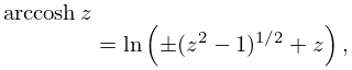
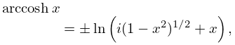
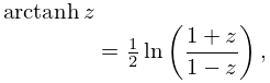
8: 4.37 Inverse Hyperbolic Functions

… ►In (4.37.2) the integration path may not pass through either of the points $\pm 1$, and the function ${(t^2-1)}^{1/2}$ assumes its principal value when $t\in (1,\mathrm{\infty })$. … ►

4.37.19 $$\mathrm{arccosh}z=\ln \left(\pm {(z^2-1)}^{1/2}+z\right),$$ $z\in ℂ\setminus (-\mathrm{\infty },1)$,

ⓘ

Symbols:

$ℂ$: complex plane, $\in$: element of, $\mathrm{arccosh}z$: inverse hyperbolic cosine function, $\ln z$: principal branch of logarithm function, $(a,b)$: open interval, $\setminus$: set subtraction and $z$: complex variable

Referenced by:

§4.37(iv), §4.37(iii), §4.37(iv)

Permalink:

http://dlmf.nist.gov/4.37.E19

Encodings:

pMML, png, TeX

See also:

Annotations for §4.37(iv), §4.37(iv), §4.37 and Ch.4

… ►It should be noted that the imaginary axis is not a cut; the function defined by (4.37.19) and (4.37.20) is analytic everywhere except on $(-\mathrm{\infty },1]$. … ►

4.37.22 $$\mathrm{arccosh}x=\pm \ln \left(\mathrm{i}{(1-x^2)}^{1/2}+x\right),$$ $x\in (-1,1]$,

ⓘ

Symbols:

$\in$: element of, $\mathrm{arccosh}z$: inverse hyperbolic cosine function, $\mathrm{i}$: imaginary unit, $\ln z$: principal branch of logarithm function, $(a,b]$: half-closed interval and $x$: real variable

Permalink:

http://dlmf.nist.gov/4.37.E22

Encodings:

pMML, png, TeX

See also:

Annotations for §4.37(iv), §4.37(iv), §4.37 and Ch.4

… ►

4.37.24 $$\mathrm{arctanh}z=\frac{1}{2}\ln \left(\frac{1+z}{1-z}\right),$$ $z\in ℂ\setminus (-\mathrm{\infty },-1]\cup [1,\mathrm{\infty })$;

ⓘ

Symbols:

$[a,b)$: half-closed interval, $ℂ$: complex plane, $\in$: element of, $\mathrm{arctanh}z$: inverse hyperbolic tangent function, $\ln z$: principal branch of logarithm function, $(a,b]$: half-closed interval, $\setminus$: set subtraction, $\cup$: union and $z$: complex variable

Permalink:

http://dlmf.nist.gov/4.37.E24

Encodings:

pMML, png, TeX

See also:

Annotations for §4.37(iv), §4.37(iv), §4.37 and Ch.4

…

9: 1.5 Calculus of Two or More Variables

… ►A function $f(x,y)$ is continuous at a point $(a,b)$ if … ► $f(x,y)$ has a local minimum (maximum) at $(a,b)$ if … ►for all $c_1\in [c_0,d)$ and all $x\in [a,b]$. … ►Let $f(x,y)$ be defined on a closed rectangle $R=[a,b]\times [c,d]$. … ►Moreover, if $a,b,c,d$ are finite or infinite constants and $f(x,y)$ is piecewise continuous on the set $(a,b)\times (c,d)$, then …

10: 4.3 Graphics

… ►

►►

Figure 4.3.1: $\ln x$ and ${\mathrm{e}}^x$. Parallel tangent lines at $(1,0)$ and $(0,1)$ make evident the mirror symmetry across the line $y=x$, demonstrating the inverse relationship between the two functions. Magnify

… ►In the labeling of corresponding points $r$ is a real parameter that can lie anywhere in the interval $(0,\mathrm{\infty })$. …