About the Project

induced%20modulus

AdvancedHelp

(0.002 seconds)

1—10 of 579 matching pages
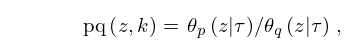
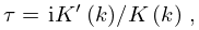
1: 22.2 Definitions
§22.2 Definitions
The nome q is given in terms of the modulus k by …
22.2.11 p q ( z , k ) = θ p ( z | τ ) / θ q ( z | τ ) ,
2: 27.8 Dirichlet Characters
A divisor d of k is called an induced modulus for χ if … where χ 0 is a character (mod d ) for some induced modulus d for χ , and χ 1 is the principal character (mod k ). …
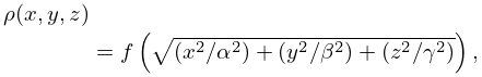
3: 19.33 Triaxial Ellipsoids
The surface area of an ellipsoid with semiaxes a , b , c , and volume V = 4 π a b c / 3 is given by … and the electric capacity C = Q / V ( 0 ) is given by … Let a homogeneous magnetic ellipsoid with semiaxes a , b , c , volume V = 4 π a b c / 3 , and susceptibility χ be placed in a previously uniform magnetic field H parallel to the principal axis with semiaxis c . The external field and the induced magnetization together produce a uniform field inside the ellipsoid with strength H / ( 1 + L c χ ) , where L c is the demagnetizing factor, given in cgs units by …
19.33.9 ρ ( x , y , z ) = f ( ( x 2 / α 2 ) + ( y 2 / β 2 ) + ( z 2 / γ 2 ) ) ,
4: Bibliography L
  • P. W. Lawrence, R. M. Corless, and D. J. Jeffrey (2012) Algorithm 917: complex double-precision evaluation of the Wright ω function. ACM Trans. Math. Software 38 (3), pp. Art. 20, 17.
  • D. J. Leeming (1977) An asymptotic estimate for the Bernoulli and Euler numbers. Canad. Math. Bull. 20 (1), pp. 109–111.
  • J. Lehner (1941) A partition function connected with the modulus five. Duke Math. J. 8 (4), pp. 631–655.
  • D. W. Lozier (1993) An underflow-induced graphics failure solved by SLI arithmetic. In IEEE Symposium on Computer Arithmetic, E. E. Swartzlander, M. J. Irwin, and G. A. Jullien (Eds.), Washington, D.C., pp. 10–17.
  • 5: 20 Theta Functions
    Chapter 20 Theta Functions
    6: 27.15 Chinese Remainder Theorem
    Their product m has 20 digits, twice the number of digits in the data. …These numbers, in turn, are combined by the Chinese remainder theorem to obtain the final result ( mod m ) , which is correct to 20 digits. Even though the lengthy calculation is repeated four times, once for each modulus, most of it only uses five-digit integers and is accomplished quickly without overwhelming the machine’s memory. …
    7: 10.75 Tables
  • The main tables in Abramowitz and Stegun (1964, Chapter 9) give J 0 ( x ) to 15D, J 1 ( x ) , J 2 ( x ) , Y 0 ( x ) , Y 1 ( x ) to 10D, Y 2 ( x ) to 8D, x = 0 ( .1 ) 17.5 ; Y n ( x ) ( 2 / π ) J n ( x ) ln x , n = 0 , 1 , x = 0 ( .1 ) 2 , 8D; J n ( x ) , Y n ( x ) , n = 3 ( 1 ) 9 , x = 0 ( .2 ) 20 , 5D or 5S; J n ( x ) , Y n ( x ) , n = 0 ( 1 ) 20 ( 10 ) 50 , 100 , x = 1 , 2 , 5 , 10 , 50 , 100 , 10S; modulus and phase functions x M n ( x ) , θ n ( x ) x , n = 0 , 1 , 2 , 1 / x = 0 ( .01 ) 0.1 , 8D.

  • Achenbach (1986) tabulates J 0 ( x ) , J 1 ( x ) , Y 0 ( x ) , Y 1 ( x ) , x = 0 ( .1 ) 8 , 20D or 18–20S.

  • Makinouchi (1966) tabulates all values of j ν , m and y ν , m in the interval ( 0 , 100 ) , with at least 29S. These are for ν = 0 ( 1 ) 5 , 10, 20; ν = 3 2 , 5 2 ; ν = m / n with m = 1 ( 1 ) n 1 and n = 3 ( 1 ) 8 , except for ν = 1 2 .

  • Bickley et al. (1952) tabulates x n I n ( x ) or e x I n ( x ) , x n K n ( x ) or e x K n ( x ) , n = 2 ( 1 ) 20 , x = 0 (.01 or .1) 10(.1) 20, 8S; I n ( x ) , K n ( x ) , n = 0 ( 1 ) 20 , x = 0 or 0.1 ( .1 ) 20 , 10S.

  • The main tables in Abramowitz and Stegun (1964, Chapter 9) give e x I n ( x ) , e x K n ( x ) , n = 0 , 1 , 2 , x = 0 ( .1 ) 10 ( .2 ) 20 , 8D–10D or 10S; x e x I n ( x ) , ( x / π ) e x K n ( x ) , n = 0 , 1 , 2 , 1 / x = 0 ( .002 ) 0.05 ; K 0 ( x ) + I 0 ( x ) ln x , x ( K 1 ( x ) I 1 ( x ) ln x ) , x = 0 ( .1 ) 2 , 8D; e x I n ( x ) , e x K n ( x ) , n = 3 ( 1 ) 9 , x = 0 ( .2 ) 10 ( .5 ) 20 , 5S; I n ( x ) , K n ( x ) , n = 0 ( 1 ) 20 ( 10 ) 50 , 100 , x = 1 , 2 , 5 , 10 , 50 , 100 , 9–10S.

  • 8: 9.18 Tables
  • Miller (1946) tabulates Ai ( x ) , Ai ( x ) for x = 20 ( .01 ) 2 ; log 10 Ai ( x ) , Ai ( x ) / Ai ( x ) for x = 0 ( .1 ) 25 ( 1 ) 75 ; Bi ( x ) , Bi ( x ) for x = 10 ( .1 ) 2.5 ; log 10 Bi ( x ) , Bi ( x ) / Bi ( x ) for x = 0 ( .1 ) 10 ; M ( x ) , N ( x ) , θ ( x ) , ϕ ( x ) (respectively F ( x ) , G ( x ) , χ ( x ) , ψ ( x ) ) for x = 80 ( 1 ) 30 ( .1 ) 0 . Precision is generally 8D; slightly less for some of the auxiliary functions. Extracts from these tables are included in Abramowitz and Stegun (1964, Chapter 10), together with some auxiliary functions for large arguments.

  • Fox (1960, Table 3) tabulates 2 π 1 / 2 x 1 / 4 exp ( 2 3 x 3 / 2 ) Ai ( x ) , 2 π 1 / 2 x 1 / 4 exp ( 2 3 x 3 / 2 ) Ai ( x ) , π 1 / 2 x 1 / 4 exp ( 2 3 x 3 / 2 ) Bi ( x ) , and π 1 / 2 x 1 / 4 exp ( 2 3 x 3 / 2 ) Bi ( x ) for 3 2 x 3 / 2 = 0 ( .001 ) 0.05 , together with similar auxiliary functions for negative values of x . Precision is 10D.

  • Zhang and Jin (1996, p. 337) tabulates Ai ( x ) , Ai ( x ) , Bi ( x ) , Bi ( x ) for x = 0 ( 1 ) 20 to 8S and for x = 20 ( 1 ) 0 to 9D.

  • Miller (1946) tabulates a k , Ai ( a k ) , a k , Ai ( a k ) , k = 1 ( 1 ) 50 ; b k , Bi ( b k ) , b k , Bi ( b k ) , k = 1 ( 1 ) 20 . Precision is 8D. Entries for k = 1 ( 1 ) 20 are reproduced in Abramowitz and Stegun (1964, Chapter 10).

  • Sherry (1959) tabulates a k , Ai ( a k ) , a k , Ai ( a k ) , k = 1 ( 1 ) 50 ; 20S.

  • 9: 19.25 Relations to Other Functions
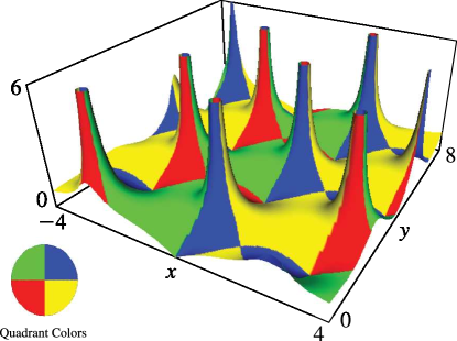
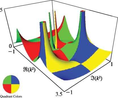
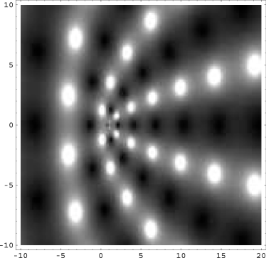
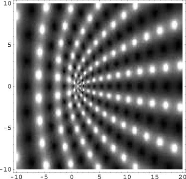
    Let k 2 = 1 k 2 and c = csc 2 ϕ with 0 ϕ π / 2 . … then the five nontrivial permutations of x , y , z that leave R F invariant change k 2 ( = ( z y ) / ( z x ) ) into 1 / k 2 , k 2 , 1 / k 2 , k 2 / k 2 , k 2 / k 2 , and sin ϕ ( = ( z x ) / z ) into k sin ϕ , i tan ϕ , i k tan ϕ , ( k sin ϕ ) / 1 k 2 sin 2 ϕ , i k sin ϕ / 1 k 2 sin 2 ϕ . Thus the five permutations induce five transformations of Legendre’s integrals (and also of the Jacobian elliptic functions). … Let r = 1 / x 2 . … where we assume 0 x 2 1 if x = sn , cn , or cd ; x 2 1 if x = ns , nc , or dc ; x real if x = cs or sc ; k x 1 if x = dn ; 1 x 1 / k if x = nd ; x 2 k 2 if x = ds ; 0 x 2 1 / k 2 if x = sd . …
    10: 22.3 Graphics
    §22.3(iv) Complex k
    See accompanying text
    Figure 22.3.24: sn ( x + i y , k ) for 4 x 4 , 0 y 8 , k = 1 + 1 2 i . … Magnify 3D Help
    See accompanying text
    Figure 22.3.25: sn ( 5 , k ) as a function of complex k 2 , 1 ( k 2 ) 3.5 , 1 ( k 2 ) 1 . … Magnify 3D Help
    See accompanying text
    Figure 22.3.26: Density plot of | sn ( 5 , k ) | as a function of complex k 2 , 10 ( k 2 ) 20 , 10 ( k 2 ) 10 . … Magnify
    See accompanying text
    Figure 22.3.27: Density plot of | sn ( 10 , k ) | as a function of complex k 2 , 10 ( k 2 ) 20 , 10 ( k 2 ) 10 . … Magnify